It is often claimed animals are more sample efficient, meaning that they can learn from many fewer examples (sometimes from single examples), than artificial neural networks and that one of the reasons for this is the useful innate inductive biases sculpted into the brains of animals through adaptations over evolutionary time scales. This claim is then usually followed by a prescriptive advice that we do something similar with artificial neural networks, namely, build in more innate structure into our models (or at least include an outer optimization loop in our models that would learn such useful inductive biases over longer time scales, as in meta-learning). Tony Zador and Gary Marcus made arguments of this sort recently.
In this post, I’d like to take issue with arguments of this sort. Actually, my objection to these kinds of arguments is already well-known. Zador has a section in his paper addressing precisely this objection (the section is titled “supervised learning or supervised evolution?”). So, what is the objection? The objection is that arguments of this sort conflate biology and simulation. They assume that the learning that happens in an artificial neural network is comparable to the learning that happens in a biological system over its individual lifespan. But there’s no good reason to think of artificial learning in this way. We should rather think of it as a combination of the learning that happens over an individual lifespan and the adaptations that take place over evolutionary time scales. When we think of artificial learning in this light, the sample efficiency argument in favor of animals falls by the wayside, because biological evolution has been running the most intense optimization algorithm in the biggest and the most detailed simulation environment ever (called “the real world”) for billions of years (so much for “one-shot” learning).
As I said, Zador is aware of this objection, so what is his response to it? As far as I can tell, he doesn’t really have a very convincing response. He correctly points out the differences between biological optimization and learning in artificial networks, but this doesn’t mean that they can’t generate functionally equivalent networks.
For example, Zador notes that biological optimization runs two nested optimization loops, the inner loop characterizing the learning processes in individual lifespans, the outer loop characterizing the adaptations over evolutionary time scales. This is similar to a learning paradigm called meta-learning in machine learning. And because of its similarity to biology, Zador is very much sympathetic to meta-learning. But in my mind the jury is still out on whether meta-learning has any significant advantages over other standard learning paradigms in machine learning. There are recent results suggesting that in practical problems one doesn’t really need the two separate optimization loops in meta-learning (one loop is all you need!). Moreover, if one trains one’s model in a sufficiently diverse range of problems (but crucially using a standard learning paradigm, such as supervised learning or reinforcement learning), “meta-learning” like effects emerge automatically without any need for two separate optimization loops (see also this beautiful new theory paper explaining some of these experimental results).
The core problem here, I think, is again conflating biology and simulation. Just because we see something in biology doesn’t mean we should emulate it blindly. Biology is constrained in many ways simulation isn’t (and vice versa). Of course it makes sense to use two separate optimization loops in biology, because individual lifespans are limited, but this isn’t true in simulation. We can run our models arbitrarily long on arbitrarily many tasks in simulation.
I think this (i.e. the mismatch between biology and simulation) is also why naive ways of emulating the brain’s innate inductive biases, like trying to directly replicate the concept of “cell types” in the brain is usually not very effective in artificial neural networks, because in my opinion these features are essentially consequences of the brain’s suboptimal learning algorithms (over developmental time scales), which means that it has to off-load a significant chunk of the optimization burden to evolution, which needs to craft these intricate cell types to compensate for the suboptimality of learning (over developmental time scales). Learning in artificial neural networks, on the other, is much more powerful, it is not constrained by all the things that biological learning is constrained by (for example, locality and limited individual lifespans), so it doesn’t really need to resort to these kinds of tricks (like different innate cell types) to easily learn something functionally equivalent over the individual lifespan.
In other words, does the brain have to do something like backprop? For those who are already familiar with this literature, my short answer is that no, the brain doesn’t have to do, and it probably doesn’t do, deep credit assignment. In this post, I’d like to discuss two reasons that make me think so. I should note from the outset that these are not really “knock-out” arguments, but more like plausibility arguments.
I have to first clarify what exactly I mean by “deep credit assignment” or “something like backprop”. This is still not going to be very exact, but by this I basically mean a global credit assignment scheme that propagates precise “credit signals” from elsewhere in a deep network in order to compute a local credit signal. I thus include any gradient-based method (first-, second-, or higher-order) in this category, as well as imperfect, heuristic versions of it such as feedback alignment or weight mirrors. There are some borderline cases such as decoupled neural interfaces that compute credits locally, but also learn gradient estimates over longer timescales. I’m inclined to include these in the “deep credit assignment” category as well, but I would have to think a bit more carefully about it before doing so confidently.
Now moving on to the two reasons that make me think the brain probably doesn’t do “deep credit assignment”. The first reason is this. I think it is very natural to think that the brain should be doing something like backprop, because it is what works today! Deep neural networks trained with gradient descent have been enormously successful in a variety of important and challenging tasks, like object recognition, object detection, speech recognition, machine translation etc. But it is very important to also remember that these successes depend on the current hardware technology. The methods that work well today are methods that work well on current hardware. But the current hardware technology is constrained in a variety of ways that brains aren’t.
Take the example of memory. Fast memory (for example, on-chip memory) is extremely limited in size in the current chip technology (although this may be beginning to change with novel chip designs such as Graphcore’s IPU and Cerebras’s WSE). But, there is no reason to think that the brain is limited in the same way, because the brain has a completely different computational architecture!
What is the significance of this observation? Well, even today we know that there are promising alternatives to backprop training in deep nets that are currently intractable precisely because of memory constraints: I’m thinking, in particular, of the deep nets as Gaussian processes (GPs) perspective. Amazingly, this method doesn’t require anytraining in the usual sense. Inference is accomplished through a single forward pass just like in backprop-trained nets. The catch is that, unlike in backprop-trained nets, this forward pass doesn’t scale well with the data size: it requires manipulating huge matrices. To my knowledge, these methods currently remain completely intractable for, say, ImageNet scale data, where the said matrices become terabyte-sized (there’s this recent paper that carries out exact GP computations on a million data points, but they use low-dimensional datasets and they don’t use deep-net kernels in their experiments; exact GPs on high-dimensional data using deep-net kernels remain highly intractable, to the best of my knowledge).
As a side note here, I would like to express my gut feeling that there may be more tractable versions of this idea (i.e. training-free or almost training-free deep nets) that are not being explored thoroughly enough by the community. One simple idea that I have been thinking about recently is the following. Suppose we take the architecture of your favorite deep neural network and set the parameters of this network layer by layer using only information inherent in the training data, say, a large image dataset. This would work as follows. Suppose the network has k filters in its first (convolutional) layer. Then we can either crop k random patches of the appropriate size from the training images or maybe do something more intelligent, like exhaustively cropping all non-overlapping patches of the appropriate size and then doing something like k-means clustering to reduce the number of crops to k and then setting those to be the first layer filters. This then fixes the first layer parameters (assuming the biases are zero). We can iterate this process layer by layer, at each layer computing a number of clusters over the activations of the previous layer across the entire training data and then basically “pasting” those clusters to the layer weights. Note that in this scheme even though there is learning (after all we are using the training data), it is minimal and non-parametric (we’re doing only k-means, for example), and nothing like a gradient-based learning scheme. I think it would be interesting to find out how well one can do with a scheme like this that uses minimal learning and utilizes almost exclusively the prior information inherent in the network architecture and the training data instead.
So, this was the first reason why I think the brain probably doesn’t do something like backprop, to wit: backprop seems to me too closely wedded to the current hardware technology. My hunch is that there are many more interesting, novel (and probably more biologically plausible) ways of building intelligent systems that don’t require anything like backprop, but we’re currently not exploring or considering these because they remain intractable with current hardware (large scale GPs being one concrete example).
The second reason is that even with the current hardware we have some recent hints that purely local learning schemes that don’t require any deep credit assignment can rival the performance of backprop training in realistic tasks (and if the brain doesn’t have to do something, the chances are it’s not going to do it!). I’d like to mention two recent papers, in particular: Greedy layerwise learning can scale to ImageNet by Belilovsky et al. and Training neural networks with local error signals by Nokland and Eidnes. These papers both introduce completely local, layerwise training schemes and show that they can work as well as end-to-end backprop in standard image recognition problems.
Although these results are impressive, in a way I consider these as still initial efforts. I feel pretty confident that if more collective effort is put into this field, even better local training schemes will be discovered. So, to me these results suggest that the problems we typically solve with end-to-end deep learning these days may not be hard enough to require the full force of end-to-end backprop. Furthermore, with each new clever local learning trick, we will discover these problems to be even easier than we had imagined previously, so in the end coming full circle from a time when we had considered computer vision to be an easy problem, to discovering that it is in fact hard, to discovering that it isn’t that hard after all!
Update (01/16/2020): I just found out that the idea I described in this post for building a gradient descent-free image recognition model using k-means clustering was explored in some early work by Adam Coates and colleagues with promising results (for example, see this paper and this). They use relatively small datasets and simple models in these papers (early days of deep learning!), so maybe it is time to reconsider this idea again and try to scale it up.
Last week, a group of researchers from Google posted a paper on arxiv describing an object recognition model claimed to achieve state-of-the-art (sota) results on three benchmarks measuring out-of-sample generalization performance of object recognition models (ImageNet-A, ImageNet-C, and ImageNet-P), as well as on ImageNet itself. These claims have yet to be independently verified (the trained models have not been released yet), but the reported gains on previous sota results are staggering:
The previous sota results on ImageNet-A, ImageNet-C, and ImageNet-P were reported in a paper I posted on arxiv in July this year, and they were achieved by a large model trained by Facebook AI researchers on ~1B images from Instagram using “weak” (i.e. noisy) labels, then fine-tuned on ImageNet (these models are called ResNeXt WSL models, WSL standing for weakly supervised learning). People who have worked on these benchmarks before will appreciate how impressive these numbers are. Particularly impressive for me are the ImageNet-A results. This benchmark itself was introduced in the summer this year and given the lackluster performance of even the best ResNeXt WSL models reported in my paper, I thought it would take a while to see reasonably high accuracies on this challenging benchmark. I was spectacularly wrong!
So, how did they do it? Their method relies on the old idea of co-training: starting from a model trained on a relatively small amount of high-quality labeled examples (in this case, ImageNet trained models), they infer labels on a much larger unlabeled dataset (in this case, the private JFT-300M dataset), then they train a model on the combined dataset (labeled + unlabeled) using random data augmentation during training, then they iterate this whole process several times.
In my arxiv paper posted back in July, I had confidently claimed that:
We find it unlikely that simply scaling up the standard object classification tasks and models to even more data will be sufficient to feasibly achieve genuinely human-like, general-purpose visual representations: adversarially robust, more shape-based and, in general, better able to handle out-of-sample generalization.
Although the Google paper doesn’t use a “standard” training paradigm, I would definitely consider it pretty close (after all, they simply find a much better way to make use of the large amount of unlabeled data, bootstrapping from a relatively small amount of labeled data, otherwise the setup is a pretty standard semi-supervised learning setup). So, I would happily admit that these results at least partially disprove my claim (it still remains to be seen to what extent this model behaves more “human-like”, I would love to investigate this thoroughly once the trained models are released).
This paper also highlights a conflict that I feel very often these days (also discussed in this earlier post). Whenever I feel pretty confident that standard deep learning models and methods have hit the wall and that there’s no way to make significant progress without introducing more priors, somebody comes along and shatters this idea by showing that there’s actually still a lot of room for progress by slightly improved (yet still very generic) versions of the standard models and methods (with no need for stronger priors). I guess the lesson is that we really don’t have very good intuitions about these things, so it’s best not to have very strong opinions about them. In my mind, the empirical spirit driving machine learning these days (“just try it and see how well it works”) is probably the best way forward at this point.
Another lesson from this paper is that bootstrapping, self-training type algorithms might be powerful beyond our (or at least my) paltry imagination. GANs and self-play type algorithms in RL are other examples of this class. We definitely have to better understand when and why these algorithms work as well as they seem to do.
Update (12/03/19):Another interesting paper from Google came out recently, proposing adversarial examples as a data augmentation strategy in training large scale image recognition models. Surprisingly, this doesn’t seem to lead to the usual clean accuracy drop if the BatchNorm statistics are handled separately for the adversarial examples vs. the clean examples and the perturbation size is kept small. Interestingly for me, the paper also reports non-trivial ImageNet-A results for the large baseline EfficientNet models. For example, the standard ImageNet-trained EfficientNet-B7 model has a reported top-1 accuracy of 37.7%. This is far better than the 16.6% top-1 accuracy achieved by the largest ResNeXt WSL model. These large EfficientNet models use higher resolution images as inputs, so it seems like just increasing the resolution gains us non-trivial improvements on ImageNet-A. This doesn’t diminish the impressiveness of the self-training results discussed in the main post above, but it suggests that part of the improvements there can simply be attributed to using higher resolution images.
I should preface this post by cautioning that it may contain some premature ideas, as I’m writing this mainly to clarify my own thoughts about the topic of this post.
In a reading group on program induction, we’ve recently discussed an interesting paper by Mollica & Piantadosi on learning kinship words, e.g. father, mother, sister, brother, uncle, aunt, wife, husband etc. In this paper, they are formalizing this as a probabilistic program induction problem. This approach comes with all the benefits of explicit program-like representations: compositionality, sample efficiency, systematic generalization etc. However, I’m always interested in neurally plausible ways of implementing these types of representations. The paper discussed an earlier work by Paccanaro & Hinton, which proposes a vector space embedding approach to the same problem. So, I decided to check out that paper.
Paccanaro & Hinton model people as vectors and relations between people as matrices (so might mean “ is the father of “). The idea is then to learn vector representations of the people in the domain, , and matrix representations of the relations between them, , such that the distance between and is minimized if the corresponding relation holds between and , and maximized otherwise. This is (by now) a very standard approach to learning vector space embeddings of all sorts of objects. I have discussed this same approach in several other posts on this blog (e.g. see here and here).
Paccanaro & Hinton model each relation with a separate unconstrained matrix. Unfortunately, I think this is not really the best way to approach this problem, since it ignores a whole lot of symmetry and compositionality in relationships (which very likely negatively impacts the generalization performance and the sample efficiency of the model): for example, if is the father of , then is a son or a daughter of . Most primitive relations are actually identical up to inversion and gender. Other relations can be expressed as compositions of more primitive relations as in Mollica & Piantadosi.
So, I tried to come up with a more efficient scheme than Paccanaro & Hinton. My first attempt was to use only two primitive relations, (e.g. mother of) and (e.g. wife of) and to use matrix inversion and transpose to express the symmetric and opposite-gendered versions of a relationship. Here are some examples:
: mother
: father
: daughter
: son
: father’s mother
: mother’s father
: mother’s son(brother)
: father’s daughter(sister)
At this point, we run into a problem: mother’s daughter and father’s son always evaluate to self (the identity matrix), and this just doesn’t quite feel right. Intuitively, we feel that extensions of these concepts should include our sisters and brothers as well, not just us. The fundamental problem here is that we want at least some of these concepts to be able to pick out a set of vectors, not just a single vector; but this is simply impossible when we’re using matrices to represent these concepts (when applied to a vector, they will give back another vector). This seems like a fairly basic deficiency in the expressive power of this type of model. If anybody reading this has any idea about how to deal with this issue in the context of vector space models, I’d be interested to hear about it.
Another question is: assuming something like this is a reasonably good model of kinship relations (or similar relations), how do we learn the right concepts given some relationship data, e.g. , etc.? If we want to build an end-to-end differentiable model, one idea is to use something like a deep sparsely gated mixture of experts model where at each “layer” we pick one of our 7 primitive relations (indexed from 0 to 6):
and the specific gating chosen depends on the input and output, and , .
So, to give an example, if we allow up to 5 applications of the primitives, the output of the gating function for a particular input-output pair might be something like: or a suitable continuous relaxation of this. This particular gating expresses the relationship, , whereas would correspond to . If we use a suitably chosen continuous relaxation for the discrete gating function, the whole model becomes end-to-end differentiable and can be trained in the same way as in Paccanaro & Hinton. We can also add a bias favoring the identity primitive over the others in order to learn simpler mappings (as in Mollica & Piantadosi). It would be interesting to test how well this model performs compared to the probabilistic program induction model of Mollica & Piantadosi and compared to less constrained end-to-end differentiable models.
Update (10/11/19): There’s some obvious redundancy in the scheme for representing compositional relations described in the last paragraph: applications of the identity don’t have any effect on the resulting matrix and successive applications of and (or and ) cancel out each other. So, a leaner scheme might be to first decide on the number of non-identity primitives to be applied and generate a sequence of exactly that length using only the 6 non-identity primitives. The successive application of inverted pairs can be further eliminated by essentially hard-coding this constraint into . These details may or may not turn out to be important.
At the end of my last post, I mentioned the possibility that a large episodic memory might obviate the need for sophisticated learning algorithms. As a fun and potentially informative exercise, I decided to quantify this argument with a little experiment. Specifically, given a finite amount of data, I wanted to quantify the relative value of learning from that data (i.e. by updating the parameters of a model using that data) vs. just memorizing the data.
To do this, I compared models that employ a mixture of learning and memorizing strategies. Given a finite amount of “training” data, a k%-learner uses k% of this data for learning and memorizes the rest of the data using a simple key-value based cache memory. A 100%-learner is a pure learner that is typical in machine learning. For the learning model, I used a ResNet-32 and for the memory model, I used the cache model described in this paper. The predictions of a k%-learner are given by a linear combination of the predictions obtained from the learner (ResNet-32) and the predictions obtained from the cache memory:
prediction = w * prediction from the learning model + (1-w ) * prediction from the cache memory
where w is a hyper-parameter that is estimated separately for each k%-learner (I assume that the cost of learning a single hyper-parameter is negligible compared to the cost of learning the parameters of a model).
Suppose I already used up k% of the data for training my ResNet-32 model and this achieves a generalization accuracy of x. Now the question is: what should I do with the rest of the data? I can either use that data to continue to train my model, which leads to a 100% learner and let’s say this 100% learner achieves an accuracy of y; alternatively I can just memorize the remaining data by caching (with the help of my partially trained ResNet-32 model), which leads to a k%-learner and let’s say this k%-learner achieves an accuracy of z. Then, given that I have already used k% of the data for learning, the relative value of learning the remaining data over just memorizing it is defined by:
relative_value_of_learning(k) = (y-x) / (z-x)
that is, the improvement in accuracy achieved by a 100%-learner divided by the improvement in accuracy achieved by the k%-learner. A large value here indicates that learning is much more valuable than memorizing (i.e. it pays off to learn from the remaining data rather than just memorizing it) and a value of 1 would indicate that learning and memorizing are equally valuable. In the latter case, given that learning is usually computationally much more expensive than memorizing, we would probably be inclined to memorize rather than learn.
The following figure shows the relative_value_of_learning(k) as a function of k for the CIFAR-10 benchmark.
So, by this measure learning is ~10 times as valuable as memorizing in this task. There appears to be a decreasing trend in the value of learning as k becomes larger, but the data is a bit noisy (ideally, I should have run this simulation multiple times to get more reliable estimates).
Is this result surprising? It was surprising to me! I was expecting the relative value of learning to be smaller and the curve shown above to approach 1 much more quickly. So, now I am a bit less skeptical of the growing literature on biologically plausible analogues of backpropagation after this exercise. There is definitely a lot of value in learning good representations (much more value than I had initially thought).
Some caveats: this exercise is specific to a particular task and particular learning and memorizing models. The results might be different in different setups. Given that much of the effort in machine learning is directed toward coming up with better pure learning models (rather than better memory models), I expect that the relative value of learning estimated here is an overestimate, in the sense that one can improve the performance of memorizing models by using more sophisticated memory models than the simple key-value cache model assumed in this exercise.
Finally, an analysis like this should help us perform a cost-benefit analysis for learning vs. memorizing both in natural and artificial agents. Coming up with cost estimates is probably easier in artificial agents: for example, one can estimate the FLOPS involved in learning vs. memorizing a given amount of data; or one can include memory costs as well. Depending on our exact cost function, the optimal strategy would involve a specific mix, or a specific trajectory, of learning vs. memorizing during the lifetime of the agent.
I put “how the brain works” in quotes in the title, because it is in fact a misleading expression. There is no single way “the brain works.” There are different mechanisms the brain uses to solve different types of problems. My conjecture is specifically about object recognition type problems that current deep learning methods arguably excel at. As is well-known, the way current deep learning methods solve these types of problems is by training a very deep network with lots of labeled examples. The success of these methods has led many to think that the brain may be solving the same problem, or similar problems, in more or less the same way (same in terms of the final mechanism, not necessarily in terms of how the brain gets there). A manifestation of this way of thinking is the ongoing search for biologically plausible variants of the backpropagation algorithm, the “workhorse” of deep learning (see a recent review here), which is biologically patently unrealistic the way it is used in current deep learning models.
To be fair, there are good reasons to think like this. Deep learning models trained in this way are currently the best models of the ventral visual cortical areas in primates and just considering their zeroth-order performance, nothing else really even comes close to achieving near human or, in some cases, even super-human performance in sufficiently challenging object recognition tasks.
Of course, when we look a bit more closely, there are also very good reasons to be skeptical of the claims that these models are adequate models of the primate visual systems in general (and human visual system in particular). Chief among those reasons is the surprising (almost shocking) sensitivity of these models to adversarialandnatural perturbations, very unlike human vision. Another reason to be skeptical is that when people actually do a more fine-grained analysis of how humans vs. deep vision models perform on realistic image recognition tasks, they find significant differences between how the two behave.
In this post, I would like to add one more reason to the skeptic’s arsenal and argue that current deep learning models for object recognition behave psychologically unrealistically and that our brains don’t seem to me to be solving object recognition type problems in the same way. My argument is exceedingly simple. It’s an argument from subjective experience and it goes as follows. When I recognize an object, it usually comes with a strong sense of novelty or familiarity. When I recognize a coffee mug, for instance, I don’t just recognize it as a mug, but as this particular mug that I have seen before (maybe even as my own mug) or as a novel mug that I haven’t seen before. This sense of familiarity/novelty comes automatically, involuntarily, even when we are not explicitly trying to judge the familiarity/novelty of an object we are seeing. More controlled psychological experiments also confirm this: humans have a phenomenally good memory for familiarity with a massive capacity even in difficult one-shot settings (see e.g. this classic study by Lionel Standing or this more recent study by Tim Brady and colleagues).
In other words, our recognitions have a strong and automatic episodic component. This episodic component is mostly lacking in current deep vision models. They don’t have a natural way of telling whether an object is novel or familiar at the same time as they are performing the recognition task.
There may be indirect ways of doing this in trained networks, for example, maybe novel and familiar –i.e. training and test– objects produce different activation distributions in a trained network. I actually don’t know if this is the case or not, but my point is just that current deep vision models do not perform this computation naturally and automatically as part of the computation they perform for recognizing the objects in the first place. This appears to me to be a big difference from the way we humans seem to do similar tasks.
So, how can we add this episodic component to the current generation of deep vision models? Shameless plug: I wrote a paper on this. The solution turns out to be really simple: just cache everything you can (ideally everything you have seen so far), using sufficiently high-level features (not too low-level stuff). And use the cache while making predictions. Retrieval from the cache is essentially a form of episodic memory. This is not even a novel solution. People have been proposing similar ideas in reinforcement learning and in language modeling (in fact, my paper was directly inspired by this last paper). In my paper, I showed that this cache-based model is incredibly robust to adversarial perturbations, so much so that when using only the cache memory to make predictions, I wasn’t able to generate any convincing adversarial examples, even with very strong attack methods (similar robustness results have been demonstrated in otherpapers as well). I strongly believe such cache-based models will also be much more adequate models of the human (and primate) visual system.
In a recent interview, Geoff Hinton said something quite similar to what I have tried to argue in this post about the difference between the current generation of deep learning models and the brain (if I interpret it correctly):
The brain is solving a very different problem from most of our neural nets… I think the brain isn’t concerned with squeezing a lot of knowledge into a few connections, it’s concerned with extracting knowledge quickly using lots of connections.
I think Hinton is fundamentally right here and I think a massive episodic memory is one of the basic mechanisms the brain uses to “extract knowledge quickly using lots of connections.” Among other things, I think one of the important implications of this point of view is that the current emphasis in some circles on trying to find sophisticated and powerful learning algorithms in the brain, which I alluded to above, may be misplaced. I actually think that backpropagation is probably much more sophisticated and powerful than anything we will find in the brain. Any learning algorithm in the brain is restricted in various ways machine learning algorithms don’t have to be (e.g. locality, respecting the rules governing different cell types etc.). On the other hand, in terms of the sheer number of neurons and the sheer number of connections, the human brain is massive compared to any model we have ever trained. It seems to me that we will soon find out that the algorithms relevant for the kind of machine the brain is are much more different than the machine learning algorithms relevant for today’s piddling models (piddling relative to the size of the human brain, of course). For example, I have always thought that hashing algorithms, essential for performing similarity search over very large sets of high-dimensional objects, should be at least as important and as relevant as backpropagation (and probably more) in our quest to understand the brain. And I have at least some corroborating evidence from the fly brain, of all places!
There is a well-known argument in psychology of language put forward by Noam Chomsky called the poverty of the stimulus argument. Roughly speaking, this is the claim that the linguistic data a child receives during language acquisition are vastly incomplete and insufficient to converge on the correct grammar. This claim is then used to bolster nativist arguments to the effect that large portions of grammar must be innate, already present in the child’s brain from birth in the form of a universal grammar.
There are several problematic aspects of this line of argument. The first and probably the most obvious one is that when people make a claim like this, they rarely, if ever, quantify how much linguistic data a child actually receives during the first few years of its life. Secondly, even if one does go ahead and quantify exactly the kind and amount of data a child receives during language acquisition, one still has to do the hard work and show that convergence to the correct grammar cannot happen (or is very unlikely to happen) with relatively weak, generic biases, but instead requires strong language-specific biases (i.e. that the biases have to be in the form of some kind of universal grammar). This can be tested either with architecture-agnostic methods such as Bayesian learners or with specific learning architectures like neural networks. Perfors et al., for example, show, through the Bayesian route, that linguistic input contains enough information to favor a hierarchical (as opposed to linear or flat) grammar with no prior bias favoring hierarchical grammars, directly refuting the often-made Chomskyan claim that language learners must have a strong innate prior bias in favor of hierarchical grammars. This just demonstrates how error-prone our intuitions can be regarding the learnability or otherwise of certain structures from data without strong priors and the importance of actuallychecking what one can or cannot learn from given data.
As we are increasingly able to train very large models on very large datasets, I think we are beginning to grapple with a fundamental question about the nature of human-level or super-human intelligence: how far can we go with fairly generic, but very large architectures trained on very large datasets optimizing very generic objectives like prediction or curiosity? Is it possible to get all the way to human-level or super-human perceptual and cognitive abilities in this way, or alternatively is it necessary to incorporate strong inductive biases into the network architecture and we simply don’t know how to do this yet, both because we don’t know what the right inductive biases are and also because we don’t know how to implement them in our models? Personally, I would easily rate this as one of the most important outstanding questions in cognitive sciences and AI today.
My own thinking on this question has been evolving in the direction of the first possibility lately, i.e. that we can learn a lot more than we might naively imagine using fairly generic architectures and fairly generic unsupervised objectives. Part of the reason for this shift is a whole slew of recent work demonstrating that one can indeed learn highly non-trivial, surprising things even from relatively modest amounts of data using very generic network architectures and generic training objectives. In this post, I’d like to highlight a few of these recent results.
Building on earlier work demonstrating the power of transfer learning in language-related tasks, there has been a lot of progress this year in unsupervised pre-training of language models with large amounts of unlabeled data. For example, Radford et al. first pre-trained a large Transformer model on a language modeling task (i.e. given some prior context, predict the next token) with a relatively large dataset (see also this earlier paper by Howard & Ruder that implements essentially the same idea, but with a different model and different datasets). They then fine-tuned this pre-trained model on a variety of downstream supervised classification tasks and observed large gains in most downstream tasks over state of the art models specifically trained on those tasks. The dataset that they pre-trained the model on was a corpus of ~7000 books. Although this may seem like a big dataset (and it is big compared to the datasets typically used in NLP research), it is in fact a miniscule dataset relative to how large it could potentially be. For example, as of October 2015, Google Books contained ~25 million books, i.e. , which is about 4 orders of magnitude larger than the corpus used in this study. I’m not sure about the number of parameters in the Transformer model used in this paper, but my rough estimate would be that it must be . By comparison, the human brain has synapses. We’ve never even come close to running models this big. Now try to imagine the capabilities of a system with parameters trained on a corpus of or more books. It’s almost certain that such a system would shatter all state of the art results on pretty much any NLP benchmark that exists today. It would almost definitely lead to qualitatively recognizable improvements in natural language understanding and common-sense reasoning skills, just as today’s neural machine translation systems are recognizably better than earlier machine translation systems, due in large part to much bigger models trained on much bigger datasets.
Another conceptually similar model that has been shown to work even better is the more recent BERT model by Devlin et al. The two major innovations in this paper over the Radford et al. paper are (i) the use of a bidirectional attention model, instead of the unidirectional –strictly left-to-right– attention model used in Radford et al.; and (ii) the use of two novel unsupervised pre-training objectives. Specifically, they use a masked token prediction task, where the goal is to predict some masked word or words in a sequence, rather than the more standard left-to-right prediction task used in Radford et al. and other language modeling papers. This objective allows the bidirectional attention model to make use of both the left and the right context in order to predict the masked words. In addition, they also use a novel unsupervised next sentence prediction task, where the objective is to simply predict whether two given input sentences actually follow each other or not. Training examples for this objective can be easily generated from the corpus. The motivation behind this second objective is to force the model to learn the relationships between sentences, rather than relationships between lower-level units such as words. This second objective turns out to be crucial for significantly improved performance in question answering and natural language inference tasks. The datasets used for pre-training the model amount to the equivalent of some ~30000 books by my estimation. This is significantly bigger than the dataset used by Radford et al., however it’s still a few orders of magnitude smaller than the number of books that were available on Google Books as of October 2015.
The bidirectional BERT model significantly outperforms the Radford et al. model on the GLUE benchmark even after controlling for the model size. This suggests that although both the model architecture and the pre-training objectives in the paper are still quite generic, not all generic architectures and objectives are the same, and finding the “right” architectures and objectives for unsupervised pre-training requires careful thinking and ingenuity (not to mention a lot of trial and error).
Large-scale study of curiosity-driven learning is another paper that came out this year demonstrating the power of unsupervised learning in reinforcement learning problems. In this quite remarkable paper, the authors show that an agent receiving absolutely no extrinsic reward from the environment (not even the minimal “game over” type terminal reward signal) and instead learning entirely based on an internally generated prediction error signal can learn useful skills in a variety of highly complex environments. The prediction error signal here is the error of an internal model that predicts a representation of the next state of the environment given the current observation and the action taken by the agent. As the internal model is updated over training to minimize the prediction error, the agent takes actions that lead to more unpredictable or uncertain states. One of the important messages of this paper is, again, that not all prediction error signals, hence not all training objectives, are equal. For example, trying to predict the pixels or, in general, some low-level representation of the environment doesn’t really work. The representations have to be sufficiently high-level (i.e. compact or low-dimensional). This is consistent with the crucial importance of the high-level next sentence prediction task in the BERT paper reviewed above.
As the authors note, however, this kind of prediction error objective can suffer from a severe pathology, sometimes called the noisy TV problem (in the context of this paper, this problem can be more appropriately called a “pathological gambling” problem): if the agent itself is a source of stochasticity in the environment, it may choose to exploit this to always choose actions that lead to high-entropy “chancy” states. This strategy may in turn lead to pathological behaviors completely divorced from any external goals or objectives relevant to the task or tasks at hand. The authors illustrate this kind of behavior by introducing a “noisy TV” in one of their tasks and allowing the agent to change the channel on the TV. Predictably, the agent learns to just keep changing the channel, without making any progress in the actual external task, because this strategy produces high-entropy states that can be used to keep updating its internal model, i.e. an endless stream of “interesting”, unpredictable states (incidentally, this kind of pathological behavior seems to be common in humans as well).
Once more, this highlights the importance of choosing the right kind of unsupervised learning objective that would be less prone to such pathologies. One simple way to reduce this kind of pathology might be to yoke the intrinsic reward of prediction error to whatever extrinsic reward is available in the environment: for example, one may value the intrinsic reward only to the extent that it leads to an increase in the extrinsic reward after some number of actions.
To summarize the main points I’ve tried to make in this post and to conclude with a few final thoughts:
Unsupervised learning with generic architectures and generic training objectives can be much more powerful than we might naively think. This is why we should refrain from making a priori judgments about the learnability or otherwise of certain structures from given data without hard empirical evidence.
I predict that as we apply these approaches to ever larger models and datasets, the capabilities of the resulting systems will continue to surprise us.
Although fairly generic architectures and training objectives have so far worked quite well, not all generic training objectives (and architectures) are the same. Some work demonstrably better than others. Finding the right objectives (and architectures) requires careful thinking and a lot of trial and error.
One general principle, however, seems to be that one should choose objectives that force the model to learn high-level features or variables in the environment and the relationships between them. Understanding more rigorously why this is the case is an important question in my opinion: are low-level objectives fundamentally incapable of learning the kinds of things learnable through high-level objectives or is it more of a sample efficiency problem?
In addition to the examples given above, another great example of the importance of this general principle is the generative query network (GQN) paper by Deepmind, where the authors demonstrate the power of a novel objective that forces the model to learn the high-level latent variables in a visual scene and relationships between those variables. More specifically, the objective proposed in this paper is to predict what a scene would look like from different viewpoints given its appearance from a single viewpoint. This is a powerful objective, since it requires the model to figure out the 3d geometry of the scene, properties of the objects in the scene and their spatial relationships with each other etc. from a single image. Coming up with similar objectives in other domains (e.g. in language) is, I think, a very interesting problem.
Probing the capabilities of the resulting trained systems in detail to understand exactly what they can or cannot do is another important problem, I think. For example, do pre-trained language models like BERT display compositionality? Are they more or less compositional than the standard seq2seq models? Etc.
Update:Here‘s an accessible NY Times article on the recent progress in unsupervised pre-training of language models.
Update (01/07/19): Yoav Goldberg posted an interesting paper evaluating the syntactic abilities of the pre-trained BERT model discussed in this post on a variety of English syntactic phenomena such as subject-verb agreement and reflexive anaphora resolution, concluding that “BERT model performs remarkably well on all cases.”
Training of recurrent neural networks (RNNs) suffers from the same kind of degeneracy problem faced by deep feedforward networks. In fact, the degeneracy problem is likely compounded in RNNs, because empirically the spectral radius of tends to be much larger than the spectral radius of where are random matrices drawn from the same ensemble (e.g. random Gaussian). I don’t know of a rigorous proof of this claim for random matrices (although, heuristically, it is easy to see that something like this should be true for random scalars: , but for –this is essentially the difference between a true random walk vs. a biased random walk (I thank Xaq Pitkow for pointing this out to me)–; exponentiating both sides, we can then see that the product of random scalars should be exponentially larger than the -th power of a random scalar), but this empirical observation would explain why training linear RNNs would be harder than training deep feedforward networks and one can reasonably expect something like this to hold approximately in the nonlinear case as well.
Researchers have developed methods to deal with this degeneracy problem, hence to overcome training difficulties in RNNs. One of the most well-known of these methods is the identity initialization for the recurrent weight matrix. Others proposed constraining the weight matrix to always be orthogonal, instead of orthogonalizing it at initialization only. The logic behind both of these methods is that since orthogonal transformations are isometries of the Euclidean space, applying a bunch of these transformations in a cascade does not lead to a degeneration of the metric (by “degeneration” here, I mean the collapse of the metric along the overwhelming majority of the directions in the input space and the astronomical expansion of the metric along a very small number of remaining directions). This is guaranteed in the linear case and, again, one hopes and expects (with some justification) that things are not all that different in the nonlinear case as well. So, in other words, a sequence of orthogonal transformations propagate vectors in Euclidean space without distortion, i.e. without changing their norms or the distances between them.
This is all true and fine, however, this analysis ignores a crucial factor that is relevant in training neural networks, namely the effect of noise. Noise comes in both through the stochasticity of SGD and sometimes through direct noise injection (as in Dropout) for regularization purposes. It is a bit hard to precisely characterize the noise that arises due to SGD, but let us assume for the sake of simplicity that the noise is additive so that what we propagate in the end is some kind of “signal + noise”. Now, although it is true that orthogonal transformations propagate the signal without distortion, they also propagate the noise without distortion as well. But, ultimately, we probably want a transformation that maximizes something like the signal-to-noise ratio (SNR) of the propagated signal + noise. Then, it is no longer obvious that orthogonal transformations are optimal for this purpose, because, one can, for example, imagine transformations that would amplify the signal more than they would amplify the noise (hence distorting both the signal and the noise), thus yielding a better SNR than an orthogonal transformation.
And indeed it turns out that for linear systems with additive Gaussian noise, one can mathematically show that optimal transformations (in the sense of maximizing the total SNR of the propagated signal + noise) are not orthogonal. In fact, one can say something even stronger: any optimal transformation has to be non-normal (a normal matrix is a unitarily diagonalizable matrix; all orthogonal matrices are normal, but the reverse is not true). This is the main result of this beautiful and insightful paper by Surya Ganguli and colleagues. Perhaps the simplest example of an optimal transformation in this sense is a feedforward chain: , where is the Kronecker delta function. This particular example maximizes the total SNR through a mechanism known as transient amplification: it exponentially amplifies the norm of its input transiently before the norm eventually decays to zero.
This brings me to the main message of this post: that the commonly used orthogonal initializations for recurrent neural networks are likely suboptimal because of the often neglected effect of noise. Another evidence for this claim comes from looking at the trained recurrent connectivity matrices in tasks that require memory. In this work (currently under review), we have shown that the trained recurrent connectivity matrices in such tasks always end up non-normal, with a feedforward structure hidden in the recurrent connectivity, even when they are initialized with an approximately normal matrix. How non-normal the trained matrices end up depend on a wide range of factors and investigating those factors was the main motivation for our paper. So, initializing RNNs with a non-normal matrix would potentially be a useful inductive bias for these networks.
In ongoing work, I have been investigating the merits of various non-normal initialization schemes for non-linear RNNs. One particular non-normal initialization scheme that seems to work quite well (and that is very easy to implement) is combining an identity matrix (or a scaled identity matrix) with a chain structure (which was shown by Ganguli et al. to be optimal in the case of a linear model with additive Gaussian noise). More details on these results will be forthcoming in the following weeks, I hope. Another open question at this point is whether non-normal initialization schemes are also useful for the more commonly used gated recurrent architectures like LSTMs or GRUs. These often behave very differently than vanilla recurrent networks, so I am not sure whether non-normal dynamics in these architectures will be as useful as it is in vanilla RNNs.
Update (06/15/19): Our work on a new non-normal initialization scheme for RNNs described in this post is now on arxiv. The accompanying code for reproducing some of the results reported in the paper is available in this public repository.
Perhaps the most important factor determining how quickly a neural network trains and how well it generalizes beyond the range of data it receives during training is the inductive biases inherent in its architecture. If the inductive biases embodied in the architecture match the kind of data the network receives, that can enable it to both train much faster and generalize much better. A well-known example in this regard is the convolutional architecture of the modern neural network models for vision tasks. The convolutional layers in these models implement the assumption (or the expectation) that the task that the model attempts to solve is more or less translation invariant (i.e. a given feature, of any complexity, can appear anywhere in the image). A more recent example is the relational inductive biases implemented in relational neural networks. Mechanistically, this is usually implemented with an inner-product like mechanism (sometimes also called attention) that computes an inner-product like measure between different parts of the input (e.g. as in this paper) or with a more complex MLP-like module with shared parameters (e.g. as in this paper). This inductive bias expresses the expectation that interactions between features (of any complexity) are likely to be important in solving the task that the model is being applied to. This is clearly the case for obviously relational VQA tasks such CLEVR, but may be true even in less obvious cases such as the standard ImageNet classification task (see the results in this paper).
Coming up with the right inductive biases for a particular type of task (or types of tasks) is not always straightforward and it is, in my mind, one of the things that make machine learning a creative enterprise. Here, by the “right inductive biases”, I mean inductive biases that (i) only exploit the structure in the problem (or problems) we are interested in and nothing more or less, but (ii) are also flexible enough that if the same model is applied to a problem that doesn’t display the relevant structure exactly, the model doesn’t break down disastrously (some “symbol”-based neural machines may suffer from such fragility).
In this post, I’d like to briefly highlight two really nice recent papers that introduce very simple inductive biases that enable neural networks to train faster and generalize better in particular types of problems.
The first one is from Uber AI: An intriguing failing of convolutional neural networks and the CoordConv solution. In this paper, the authors first observe that state of the art convolutional networks fail quite badly in tasks that require spatial coordinate transformations, for example, changing from Cartesian coordinates to image-based coordinates or vice versa (e.g. given the Cartesian coordinates , draw a square of a certain size centered at ). This may not be too surprising, since convolutional networks are explicitly designed to be translation-invariant, hence to ignore any spatial information, but the authors correctly note that ignoring spatial information completely (being rigidly translation-invariant) may not always be advisable (this may lead to failures of the type mentioned in (ii) above). It is rather much better to provide the model with the spatial information and let it figure out itself how much translation-invariant it needs to be in any particular task. This is exactly what the authors do. Specifically, they provide the spatial information in an explicit format through additional (fixed) channels that represent the Cartesian coordinates of each “pixel”. For image-based tasks, one thus needs only two additional channels, representing the and coordinates of each pixel. Pictorially, their scheme, which they call CoordConv, looks like this (Figure 3 in the paper):
That’s basically it. If the task at hand is highly translation-invariant, the model can learn to set the weights coming from those two Cartesian coordinate channels to small values; if the task at hand requires precise spatial information, on the other hand, the model can learn to utilize those channels appropriately. NLP people may recognize the conceptual similarity of this scheme to the positional encodings of items in sequence-based tasks. For the NLP people, we may thus summarize their contribution by saying that they extend the positional encoding idea from the temporal domain (in sequence-based tasks) to the spatial domain (in image-based tasks). It’s always a good idea to think about such exchanges between different domains!
The authors then go on to demonstrate that introducing a few of these CoordConv layers in standard architectures improves performance in a diverse range of tasks (but not in all tasks), including object detection, GAN training and Atari playing.
The second paper I’d like to highlight, called Neural Arithmetic Logic Units, starts from the observation that generic neural network architectures cannot generalize well in numerical tasks requiring arithmetic operations such addition, multiplication etc., even when they may successfully fit any given training data in such tasks (and sometimes they cannot even achieve that). The authors of this paper introduce very simple, elegant and easy-to-impement inductive biases that enable generic models (LSTMs and MLPs) to extrapolate from training data much better in such tasks. The basic idea is to “nudge” standard neural network operations (linear combination, pointwise nonlinearity etc.) to behave like arithmetic operators. For instance, for addition, they parametrize a dense weight matrix as:
where denotes elementwise multiplication, and is the sigmoid nonlinearity. In the saturated regime, this parametrization encourages to have entries, , and so a linear combination using this kind of , i.e. , tends to behave like an addition or subtraction of its inputs (without scaling). In light of the preceding discussion, it is important to note here again that the model does not force this kind of behavior, but rather it merely facilitates it.
As an inductive bias for multiplication, they use the exponentiated sum of logs formulation:
using the same matrix as above. This (approximately) expresses the multiplication of the elements in . A linear combination of these addition and multiplication operations gated by a sigmoid unit (called a NALU in the paper) then can function as either an addition or a multiplication operation (which can be learned as appropriate). One can then stack these operations to express, in principle, arbitrarily complex arithmetic operations.
This beautiful, simple idea apparently works fantastically well! I was quite impressed by the results in the paper. However, I would have liked to see (i) some results with more complex arithmetic operations than they report in the paper and also (ii) some results with tasks that do not have a strong arithmetic component to gauge how strong the introduced arithmetic inductive biases are. Again, the idea is to see whether, or how badly, the model fails when faced with a task without a strong arithmetic component. Ideally, we would hope that the model does not fail too badly in such cases.
Note: I will collect, and report here, examples of inductive biases, like the ones I discussed in this post, that I encounter in the literature, with brief descriptions of the bias introduced, how it is supposed to work and what kinds of problem it is intended to be applied to. To facilitate this, I tagged this post with the tag inductive biases and I will file similar posts under the same tag in the future.
Inspired by this thread from Ian Goodfellow, I recently finished reading a nice introductory textbook on nonstandard analysis, Infinitesimal Calculus, and I’d like to summarize here what I’ve learnt from the book.
There is a well-known construction of real numbers from rational numbers that defines real numbers as equivalence classes of Cauchy sequences of rational numbers. Two Cauchy sequences of rational numbers are counted as equal if their difference converges to zero in the Euclidean metric (choosing other metrics here gives rise to some interesting, alternative number systems, e.g. p-adic numbers).
In an analogous fashion, one can define a new number system starting from the reals this time. This new number system, called hyperreal numbers (), is defined in terms of equivalence classes of sequences of real numbers. Two sequences of real numbers, and , are considered equal (hence represent the same hyperreal number) iff the set of indices where they agree, , is quasi-big. The technical definition of a quasi-big set is somewhat complicated, but the most important properties of quasi-big sets can be listed as follows:
No finite set is quasi-big.
If and are quasi-big sets, then so is .
If is quasi-big and , then is also quasi-big.
For any set , either or its complement is quasi-big.
Given this definition of hyperreal numbers, the following properties can be established relatively straightforwardly:
, i.e. hyperreals strictly contain the reals (we map any real to the equivalence class containing the sequence ).
contains an infinitesimal, i.e. a number such that , yet for every positive real number (to see this, consider the sequence ).
In a formal language that is expressive enough to develop the entire calculus in, any given sentence is true with respect to iff it is true with respect to . This is an extremely useful property that can be derived from Łoś’s Theorem.
At this point, you might be (and you should be!) wondering whether Properties 2 and 3 above are consistent with each other. Property 2 says there’s an infinitesimal number in , but we know that there’s no infinitesimal number in . So, how is it possible that every sentence true in is also true in ? The answer is that the language mentioned in Property 3, although powerful enough to allow us to do calculus, is a rather restricted language. In particular, it doesn’t allow us to define what a real number is. This is because the definition of a real number crucially relies on the completeness axiom. The completeness axiom cannot be expressed in , because it requires talking about sets of numbers, something that turns out not to be possible in the language . So, Property 2 cannot be expressed in the language , hence is not powerful enough to distinguish hyperreals from reals.
Here are some further useful properties of hyperreal numbers:
We mentioned above that there is at least one infinitesimal hyperreal. Are there more? Yes, definitely! There are in fact an infinite number of them: for, if is an infinitesimal and is a real number, then is also infinitesimal. Moreover, if and are infinitesimals, then so are and .
We say that a hyperreal is infinite iff it is either greater than all real numbers or smaller than all real numbers. A hyperreal is finite iff it is not infinite. It is easy to show that if is infinitesimal, is an infinite hyperreal.
contains infinite integers. The proof is very easy, using Property 3 above. We know that for any in , there is an integer greater than (note that one can express this statement in the language , because “ is an integer”, unlike “ is a real”, can be defined in ). Since this is true for , it must be true for as well. In particular, there must be an integer greater than . But we just observed that is infinite, hence that integer must be infinite too! In fact, it immediately follows that there must be an infinite number of infinite integers.
We say that two hyperreals and are infinitely close, denoted by , if is infinitesimal or zero.
Let’s say that a hyperreal is nonstandard if is not real. Then, it’s easy to show that for any real and nonstandard , (or ) is nonstandard.
If is any finite hyperreal, then there exists a unique real infinitely close to
One can develop the entire calculus using hyperreal numbers, instead of the reals. This is sometimes very useful, as some results turn out to be much easier to state and prove in than in and we know, by Property 3 above, that we won’t ever be led astray by doing so. Just to give a few examples: in , we can define a function to be continuous at iff implies . In , on the other hand, we would have to invoke the notion of a limit to define continuity, which in turn is defined in terms of a well-known -type argument.
Using hyperreals, derivatives are also very easy to define. The derivative of a function at is defined as:
where is an infinitesimal (it’s easy to check that the definition doesn’t depend on which infinitesimal is chosen). Again, the definition of a derivative in standard analysis would involve limits.
Taking the derivatives of specific functions is equally easy, since we can manipulate infinitesimals just like we manipulate real numbers (again by Property 3 above).
One important difference between and is that is complete (in fact, the construction of reals as equivalence classes of Cauchy sequences of rationals, which was mentioned at the beginning of this post, is known as the completion of rationals with respect to the Euclidean metric), whereas is not complete. As mentioned before, this is not inconsistent with Property 3 above, because completeness cannot be expressed in the language .
Bonus: I recently discovered this video of a great lecture by Terry Tao on ultraproducts. Ultraproduct is the required technical concept I glossed over above when I defined quasi-bigness. Most of the lecture is quite accessible and I recommend it to anybody who wants to learn more about this topic.
One of the most important outstanding theoretical issues in machine learning today is explaining generalization in deep neural networks. Despite the fact that these models sometimes contain several orders of magnitude more parameters than the number of data points they are trained on, they do not seem to overfit the data easily and they are able to generalize successfully to new data. This highly over-parametrized regime makes the generalization error bounds derived with standard tools in statistical learning theory mostly vacuous. So, coming up with new theoretical ideas that can give non-vacuous quantitative bounds on the generalization performance of deep neural networks has been a top priority in theoretical machine learning in recent years.
There is a fair amount of empirical observation in the literature on what makes a neural network generalize better or worse. These empirical observations typically report significant correlations between the generalization performance of models on a test set and some measure of their noise robustness or degeneracy. For example, Morcos et al. (2018) observe that models that generalize better are less sensitive to perturbations in randomly selected directions in the network’s activity space. Similarly, Novak et al. (2018) observe that models that generalize better have smaller mean Jacobian norms, , than models that don’t generalize well. The Jacobian norm at a given point can be considered as an estimate of the average sensitivity of the model to perturbations around that point. So, similar to Morcos et al.’s observation, this result amounts to a correlation between the model’s generalization performance and a particular measure of its noise robustness. Wu et al. (2017) observe that models that generalize better have smaller Hessian norms (Frobenius) than models that don’t generalize well. The Hessian norm can be considered as a measure of the total degeneracy of the model, i.e. the flatness of the loss landscape around the solution. Hence this result is in line with earlier hypotheses (by Hochreiter & Schmidhuber and by Hinton & Van Camp) about a possible connection between the generalization capacity of neural networks and the local flatness of the loss landscape. For two-layer shallow networks, Wu et al. also establish a link between the noise robustness of the models as measured by their mean Jacobian norm and the local flatness of the loss landscape as measured by the Hessian norm (in a nutshell, under some fairly plausible assumptions, the mean Jacobian norm can be upper-bounded by the Hessian norm -see Corollary 1 in the paper-).
Although these observations are all informative, they do not provide a rigorous quantitative explanation for why heavily over-parametrized neural networks generalize as well as they do in practice. Such an explanation would take the form of a rigorous quantitative bound on the generalization error of a model given what we know about the model’s various properties. As I mentioned above, standard theoretical tools have so far not been able to yield non-vacuous, i.e. meaningful, bounds on generalization error for models operating in the highly over-parametrized regime.
In this post, I’d like to highlight a recent paper by Wenda Zhou and colleagues that was able to derive non-vacuous generalization error bounds for ImageNet-scale models for the first time. Following prior work by Dziugaite & Roy, their starting point is PAC-Bayes theory. They leverage the compressibility of the trained deep neural nets to derive a non-vacuous (but still very loose) PAC-Bayes bound on the generalization error of large-scale image recognition models.
Roughly speaking, PAC-Bayes theory gives bounds on the generalization error that are of the following form: , where is the number of training points, is a data-dependent posterior distribution over the “hypotheses” (think of a distribution over neural network parameters) specific to a learning algorithm and training data and is a data-independent prior distribution over the hypotheses. The main challenge in coming up with useful bounds in this framework is finding a good prior that would minimize the -divergence between the prior and the posterior in the bound. This basically requires guessing what kinds of structure are favored by the training algorithm, training data and model class we happen to use (previously, Dziugaite & Roy had directly minimized the PAC-Bayes bound with respect to the posterior distribution instead of guessing an appropriate prior, assuming a Gaussian form with diagonal covariance for the posterior, and came up with non-vacuous and fairly tight bounds for MNIST models. Although this is a clever idea, it obscures which properties of trained neural nets specifically lead to better generalization).
The main idea in the paper by Wenda Zhou and colleagues is to choose such that greater probability mass is assigned to models with short code length, i.e. more compressible models. This implicitly expresses the hypothesis that neural networks trained with SGD on real-world datasets are more likely to yield compressible solutions. When we choose and , where denotes the number of bits required to describe the model according to some pre-specified compression scheme and denotes the compressed version of the trained model, we get a bound like the following (Theorem 4.1 simplified):
This means that the more compressible the model is, the better the generalization error bound will be. The authors then refine this bound by making the compression scheme more explicit and also incorporating the noise robustness property of the trained networks into the bound. I won’t go into those details here, but definitely do check out the paper if you are interested. They then apply a state-of-the-art compression method (based on dynamic network surgery) to pre-trained deep networks to instantiate the bound. This gives non-vacuous but still very loose bounds for models trained on both MNIST and ImageNet. For example, for ImageNet, they obtain a top-1 error bound of , whereas their compressed model achieves an actual error of on the validation data.
So, although it is encouraging to get a non-vacuous bound for an ImageNet model for the first time, there is still a frustratingly large gap between the actual generalization performance of the model and the derived bound, i.e. the bounds are nowhere near tight. Why is this? There are two possibilities as I see it:
The authors’ approach of using a PAC-Bayes bound based on compression is on the right track, however the current compression algorithms are not as good as they can be, hence the bounds are not as tight as they can be. If true, this would be a practically exciting possibility, since it suggests that a few orders of magnitude better compression can be achieved with better compression methods currently not yet available.
Just exploiting compression (or compression + noise robustness) will not be enough to construct a tight PAC-Bayes bound. We have to incorporate more specific properties of the trained neural networks that generalize well in order to come up with a better prior .
The second possibility would imply the existence of models that have similar training errors and are compressible to a similar extent, yet have quite different generalization errors. I’m not aware of any reports of such models, but it would be interesting to test this hypothesis.
One of my favorite papers this year so far has been this ICLR oral paper by Zhilin Yang, Zihang Dai and their colleagues at CMU. The paper is titled “Breaking the softmax bottleneck: a high-rank RNN language model” and uncovers an important deficiency in neural language models. These models typically use a softmax layer at the top of the network, mapping a relatively low dimensional embedding of the current context to a relatively high dimensional probability distribution over the vocabulary (the distribution represents the probability of each possible word in the vocabulary given the current context). The relatively low dimensional nature of the embedding space causes a potential degeneracy in the model. Mathematically, we can express this degeneracy problem as follows:
Here, is an matrix containing the log-probability of each word in the vocabulary given each context in the dataset: , where is the number of all distinct contexts in the dataset and is the vocabulary size; is an matrix containing the embedding space representations of all distinct contexts in the dataset, where is the dimensionality of the embedding space; and is an matrix containing the softmax weights.
In typical applications, and , so is a few order orders of magnitude smaller than . This means that while the right-hand side of the above equation can be full-rank, the left-hand side is rank-deficient: i.e. (we’re assuming that is larger than and , which is usually the case). This means that the model is not expressive enough to capture .
I think it is actually more appropriate to frame the preceding discussion in terms of the distribution of singular values rather than the ranks of matrices. This is because can be full-rank, but it can have a large number of small singular values, in which case the softmax bottleneck would presumably not be a serious problem (there would be a good low-rank approximation to ). So, the real question is: what is the proportion of near-zero, or small, singular values of ? Similarly, the proportion of near-zero singular values of the left-hand side, that is, the degeneracy of the model, is equally important. It could be argued that as long as the model has enough non-zero singular values, it shouldn’t matter how many near-zero singular values it has, because it can just adjust those non-zero singular values appropriately during training. But this is not really the case. From an optimization perspective, near-zero singular values are as bad as zero singular values: they both restrict the effective capacity of the model (see this previous post for a discussion of this point).
Framed in this way, we can see that the softmax bottleneck is really a special case of a more general degeneracy problem that can arise even when we’re not mapping from a relatively low dimensional space to a relatively high dimensional space and even when the nonlinearity is not softmax. I will now illustrate this with a simple example from a fully-connected (dense) layer with relu units.
In this example, we assume that the input and output spaces have the same dimensionality (i.e. , using the notation above), so there is no “bottleneck” due to a dimensionality difference between the input and output spaces. Mathematically, the layer is described by the equation: , where is relu and we ignore the biases for simplicity. The weights, , are drawn according to the standard Glorot uniform initialization scheme. We assume that the inputs are standard normal variables and we calculate the average singular values of the Jacobian of the layer, , over a bunch of inputs. The result is shown by the blue line (labeled “Dense”) below:
The singular values decrease roughly linearly up to the middle singular value, but drop sharply to zero after that. This is caused by the saturation of approximately half of the output units. Of course, the degeneracy here is not as dramatic as in the softmax bottleneck case, where more than of the singular values would have been degenerate (as opposed to roughly half in this example), but this is just a single layer and degeneracy can increase sharply in deeper models (again see this previous post for a discussion of this point).
The remaining lines in this figure show the average singular values of the Jacobian for a mixture-of-experts layer that’s directly inspired by, and closely related to, the mixture-of-softmaxes model proposed by the authors to deal with the softmax bottleneck problem. This mixture-of-experts layer is defined mathematically as follows:
where denotes the number of experts, represents the gating model for the -th expert and is the -th expert model (a similar mixture-of-experts layer was recently used in this paper from Google Brain). The mixture-of-softmaxes model proposed in the paper roughly corresponds to the case where both and are softmax functions (with the additional difference that in their model the input is first transformed through a linear combination plus tanh nonlinearity).
The figure above shows that this mixture-of-experts model effectively deals with the degeneracy problem (just like the mixture-of-softmaxes model effectively deals with the softmax bottleneck problem). Intuitively, this is because when we add a number of matrices that are each individually degenerate, the resulting matrix is less likely to be degenerate (assuming, of course, that the degeneracies of the different matrices are not “correlated” in some sense, e.g. caused by the same columns). Consistent with this intuition, we see in the above figure that using more experts (larger ) makes the model better conditioned.
However, it should be emphasized that the mixture-of-experts layer (hence the mixture-of-softmaxes layer) likely has additional benefits other than just breaking the degeneracy in the model. This can be seen by observing that setting the gates to be constant, e.g. , already effectively breaks the degeneracy:
I haven’t yet run detailed benchmarks, but it seems highly unlikely to me that this version with constant gates would perform as well as the full mixture-of-experts layer with input-dependent gating. This suggests that, in addition to breaking the degeneracy, the mixture-of-experts layer implements other useful inductive biases (e.g. input-dependent, differential weighting of the experts in different parts of the input space), so the success of this layer cannot be explained entirely in terms of degeneracy breaking. The same comment applies to the mixture-of-softmaxes model too.
Finally, I would like to point out that the recently introduced non-local neural networks can also be seen as a special case of the mixture-of-experts architecture. In that paper, a non-local layer was defined as follows:
with input-dependent gating function and expert model . The canonical applications for this model are image-based, so the layers are actually two-dimensional (a position dimension -represented by the indices – and a feature dimension -implicitly represented by the vectors , etc.-), hence the inductive biases implemented by this model are not exactly the same as in the flat dense case above, but the analogy suggests that part of the success of this model may be explained by degeneracy breaking as well.
Note: I wrote a fairly general Keras layer implementing the mixture-of-experts layer discussed in this post. It is available here. Preliminary tests with small scale problems suggest that this layer actually works much better than a generic dense layer, so I am making the code available as a Keras layer in the hope that other people will be encouraged to explore its benefits (and its potential weaknesses). I am currently working on a convolutional version of the mixture-of-experts layer. The convolutional mixture of experts models have now been implemented and uploaded to the GithHub repository together with some examples illustrating how to use these dense and convolutional mixture of experts layers.
I just read the new Nature paper by DeepMind (& UCL) on grid cells and I’d like to share my thoughts about it. Just to briefly summarize the main points of the paper, they first show that grid cell like representations emerge naturally in fairly generic recurrent neural networks trained to do certain navigation tasks and secondly, they argue that this grid-like representation of space has benefits over alternative representations when artificial agents learn to perform relatively complex, realistic navigation tasks.
I really enjoyed reading the paper. For me, the most surprising result in the paper was the model’s apparent ability to reproduce some very subtle aspects of actual grid cell phenomenology in the brain, particularly the emergence of discrete spatial scales with geometric ordering. It is not often that one gets such discrete structures when one trains neural networks on any task. The default pattern I would have predicted would rather be continuous variation in the spatial scale of grid cells, i.e. something like a uniform or normal distribution over spatial scales.
Here are some other (more critical) thoughts on the paper:
1) I found the paper frustratingly short on explanations. Yes, hexagonal grids seem to emerge in the network, but why? Some form of regularization seems to be necessary to get grid-like representations in the network, but again why? Yes, grid-like representation of space seems to be more beneficial than a place field like representation in some navigation problems in RL, again why? Unfortunately, they don’t even put forward any plausible hypotheses as to why these results are observed.
2)An ICLR paper this year reported somewhat similar (but less detailed) results on the emergence of a grid like representation of space in trained recurrent nets. There are some important differences between the setups of these two papers; for instance, the ICLR paper trains the networks on the x, y coordinates of the agent’s position, whereas in the DeepMind paper, the training signal is a population code (place field) representation of space (plus a similar population code representation of head direction). The emergent grid in the ICLR paper was a square grid, I think; so they weren’t able to explain the hexagonal grid, nor the discrete geometrically-ordered spatial scales, as far as I know. So, this difference between the training signals seems to be important in explaining the different properties of the emergent grid. I think it is really important to understand which features of the training setup or the architecture are necessary to get the biologically more realistic hexagonal grids with geometrically spaced scales: is the linear read-out important? Is the network architecture important? What kind of training signal is necessary for the emergence of a hexagonal grid? Etc.
3) The paper also claims that when provided as input to a standard RL agent (A3C), periodic grid code representations of self-location and goal location are more beneficial than place field representations of the same variables. Again, not enough control experiments were run to determine why this is the case, but there are at least two possibilities, as far as I see: (i) it could be that a grid code affords a “better” representation of space in some sense, (ii) perhaps this effect has nothing to do with the representational power of a grid code, but it’s just a training effect (i.e. this kind of representation just happens to work better when training the policy network in A3C with SGD).
I find (i) unlikely: as the grid cells themselves were trained to match place cell responses with a linear read-out, they can’t really be a better representation of space than the place cells; it can’t be the case that grid cells provide more reliable information about space than place cells, for example, because place cells are the ground truth here. It may be argued that a grid code contains more easily decodable information than a place cell code, but I don’t see how this could be possible (if anything I would actually expect the opposite; this was, in fact, one of the messages of this paper by Sreenivasan & Fiete: simply put, although a grid code can encode a lot of information, decoding that information is not straightforward).
This leaves (ii) as the likely (and less exciting) explanation. One possible reason why a grid code would be better for training the policy network could be that the activations in the grid code are less sparse than activations in a place cell code (a straightforward prediction is that the performance of the place cell network should improve with wider place fields). A crucial control sorely missing in this section was using a smooth, random, non-periodic basis (sort of like the basis that emerges in the network when it’s trained without regularization). If that works as well as the grid code, that would suggest that there’s nothing special about periodic multi-scale codes like the grid code, similar results hold for any sufficiently dense and smooth code (a less exciting conclusion than what the paper currently seems to be concluding).
4) In the RL experiments, the grid-cell network wasn’t trained end-to-end, different components of the network were trained with different objectives (for example, see Extended Data Fig. 5). Do grid cells still emerge if the entire network is trained end-to-end with the reward maximization (RL) objective? Alternatively, let’s assume that we plug a pre-trained grid-cell module to a policy network and then fine tune it with the RL objective. Are the grid cell representations in the grid cell module stable in the face of this fine-tuning? If not, that would be problematic for the claims of the paper.
5) This is really a more minor point compared to the first four points above. In training the grid-like cells in the network, the training objective they use is to match the responses of some place cells (plus some head-direction cells) which are assumed to have developed already. I think it would be much nicer and more realistic to have an unsupervised objective that would lead to the emergence of both grid cells and place cells. For justification, the authors note that place cells seem to develop earlier than grid cells; so coming up with an unsupervised objective that would reproduce this developmental order would be very interesting.
I just posted a new paper on arxiv titled “A Simple Cache Model for Image Recognition”. In this paper, I make a very basic observation: in image recognition tasks, the layers of a deep network close to the output layer contain independent, easily extractable class-relevant information that is not already contained in the output layer itself. I then propose to read out this extra information using a simple continuous key-value cache memory that is directly inspired by Grave et al. (2017), who add a similar continuous cache memory to recurrent sequence-to-sequence models.
The really nice thing about this model is that by properly setting only two hyper-parameters, it is possible to significantly improve the accuracy of a pre-trained model at test time. For example, here are some error rates on the CIFAR-10 and CIFAR-100 test sets:
where ResNet32 () is the baseline model without a cache component, ResNet32-Cache3 is a model that linearly combines the predictions of the cache component and the baseline model (as you may have guessed, represents the mixture weight of the cache component), and ResNet32-Cache3-CacheOnly () is a model that uses the predictions of the cache component only.
I also found that a cache component substantially improves the robustness of baseline models against adversarial attacks. Here are the classification accuracies of the same three models above on adversarial images generated from the CIFAR-10 test set by four different attack methods applied to the baseline ResNet32 model:
Interestingly, the cache-only model is more robust against adversarial perturbations than the other models. It is intuitively easy to understand why cache models improve robustness against adversarial examples: they effectively extend the range in the input space over which the model behaves similarly to the way it behaves near training points and recent work has shown that neural networks behave more regularly near training points than elsewhere in the input space (for example, as measured by the Jacobian norm or the number of “linear regions” in the neighborhood of a given point).
Indeed, I confirmed this by looking at the Jacobian of the models at the test points:
Both cache models reduce the mean Jacobian norm over the baseline model (a). The two cache models, however, have somewhat different characteristics: the linear-combination model (ResNet32-Cache3) has the smallest first singular value but slightly increased lower-order singular values compared to the baseline model, whereas the cache-only model reduces the singular values (and the Jacobian norms per trial) more consistently. This pattern appears to be related to the differential generalization behavior of the two models: the linear-combination cache has the higher test accuracy, but the cache-only model is more robust against adversarial perturbations. So, the conjecture is that within-sample generalization performance is mostly determined by the first singular value (or the first few singular values), whereas the out-of-sample generalization performance, e.g. sensitivity of the models against adversarial perturbations, is also significantly affected by the lower-order singular values.
In my last post, I mentioned meta-learning as a promising approach for learning useful inductive biases in neural networks. In meta-learning, several steps of a standard optimization problem are unrolled and “baked” into the computation graph. One then performs backpropagation over the entire computation graph to optimize particular parameters or hyper-parameters of interest, for example, hyper-parameters controlling the learning rate or momentum schedules or the initial parameters of the network.
One potential problem with this approach is that it becomes computationally prohibitive to unroll, and bake into the computation graph, more than a relatively small number of optimization steps, compared to the number of optimization steps or iterations one would normally perform for training the model. One might then worry that parameters or hyper-parameters optimized over this shorter horizon might not generalize well to longer horizons (the longer horizon problem is ultimately the problem we are interested in).
A new ICLR paper by Yuhuai Wu, Mengye Ren and colleagues argues that such worries are justified, at least for a certain class of meta-learning problems. They consider the problem of meta-learning the learning rate and momentum schedules in neural network training. In the first part of the paper, they approach this problem analytically by considering a noisy quadratic loss function. For this particular loss function, it turns out that one can estimate both the optimal learning rate and momentum schedules (using Theorem 1 in the paper), as well as the “greedy-optimal” learning rate and momentum schedules that minimize the one-step ahead loss function at each time step (using Theorem 2). The authors show that although the greedy-optimal strategy outperforms the optimal schedule initially during training, its final performance is substantially worse than that of the optimal strategy. The reason appears to be that the greedy-optimal strategy reduces the learning rate prematurely to be able to decrease the loss along high-curvature directions in the loss landscape quickly enough.
In the second part of the paper, a gradient-based hyper-parameter meta-learning method is shown to suffer from a similar short-horizon bias where meta-learning of the hyper-parameters controlling the learning rate schedule (i.e. the initial learning learning rate and a hyper-parameter controlling the learning rate decay over time) with a small number of unrolled optimization steps, i.e. over a short horizon, again leads to learning rates that are reduced much too quickly compared to the optimal schedule, resulting in severely suboptimal final performances.
Here are some thoughts and questions inspired by this work:
In the inner loop of their meta-learning problems, the authors only consider vanilla SGD with momentum. It is a bit unfortunate that they don’t consider the Adam algorithm (or similar algorithms) in the inner loop. I suspect that using Adam in the inner loop might ameliorate the short-horizon bias significantly, because Adam is supposed to be less sensitive to hyper-parameter choices (one might then object, with some justification, that this would be a case where meta-learning is not really needed).
Because the bias reported in the paper seems to be consistent, i.e. always in the direction of reduced learning rates, a quick fix one could imagine would be to introduce a prior that would counteract this bias by, for example, discouraging small learning rates. I’m not quite sure what the best prior to use would be in this context and I don’t know how well this would work in practice compared to the optimal learning rate schedules, but it seems like a straightforward fix that could be worth trying.
As the authors note, the short-horizon bias becomes less significant (or might even disappear) when the optimization problem is either deterministic or well-conditioned. We have previously argued that skip connections reduce degeneracies in neural networks, thereby making the optimization problem better-conditioned. It’s likely that other methods such as batch normalization have similar effects. This suggests that more realistic architectures using skip connections and batch normalization might be less prone to the short-horizon problem uncovered in this paper. It would be interesting to investigate this.
It would also be interesting to see if other kinds of meta-learning problems, for example, meta-learning a good initialization for the model parameters (as in the MAML algorithm) suffer from similar short-horizon biases.
This is just a brief post to highlight a brilliant paper I have read recently and to share some thoughts sparked off by the paper. The paper in question is Investigating human priors for playing video games by Rachit Dubey and colleagues. In this paper, the authors address a very basic question: What kinds of specific prior knowledge do humans bring to the task of learning a new video game that make them much more efficient (in terms of the amount of training experience required) than neural networks learning a similar video game through deep RL algorithms.
Their approach to this question is thoroughly (and admirably) empirical. By designing various versions of the basic game that eliminate different kinds of structure in the game, they are able to not only identify, but also quantify the relative importance of, various different regularities or meaningful structures in the game for human players. The idea is that if the removal of a particular meaningful structure or regularity in the game severely affects the learning performance of human players, then that must be an important regularity that humans rely on heavily in learning the game. Conversely, if the removal of a meaningful structure or regularity does not affect the learning performance of human players, it is reasonable to assume that that regularity is not an important part of the prior knowledge that human players bring to the learning of the new game.
Using this logic, the authors show that (i) knowledge about how to interact with objects (e.g. one can climb a ladder by pressing the up key as opposed to zigzagging left and right, one can jump over monsters by pressing the up and right (or left) keys etc.), (ii) knowledge about object affordances (e.g. platforms support walking and ladders support climbing) and object semantics (e.g. one has to avoid fires and angry-looking monsters), (iii) the concept of an object as distinct from the background and a prior that expects visually similar things to behave similarly, are all parts of the prior knowledge that people utilize (in the order of increasing importance) in learning a new game.
One might naively think that it should be a great idea to build all this prior knowledge in our neural networks (if only we knew how to do that!). That would be expected to greatly increase the sample efficiency of neural networks when they encounter similar problems. However, one has to be careful here, since building in any kind of prior knowledge always comes at a cost: namely, if the problems encountered by the model do not conform to the assumed prior, the prior, rather than improving the sample efficiency, may in fact worsen it. The authors are (again, admirably) very clear about this potential drawback of prior knowledge (which they illustrate with a simple example video game):
However, being equipped with strong prior knowledge can sometimes lead to constrained exploration that might not be optimal in all environments… Thus, while incorporating prior knowledge in RL agents has many potential benefits, future work should also consider challenges regarding under-constrained exploration in certain kinds of settings.
Building in too many human priors could also make models vulnerable to a sort of “adversarial attack” where an adversary might design “unnatural” versions of a task that would be difficult to solve for a model with a lot of human priors (similar to the games created in the paper), a sort of inverse-CAPTCHA. A less constrained model with fewer human priors would be less vulnerable to such attacks. Besides, although human priors (especially more general ones such as the concept of an object or the visual similarity prior) are probably broadly useful in vision- or language-related problems, increasingly many problems we face today in applied sciences are not obviously amenable to any kind of useful human prior: problems in bioinformatics or molecular design come to mind, for example. Trying to prematurely incorporate human priors in our models (whatever they might be) may hinder performance in such cases. Furthermore, human priors (especially more specific ones such as those that arise in naive physics or in naive psychology) are often plain wrong, in which case incorporating them in our models doesn’t make any sense.
This is where the importance of meta-learning comes in, I think. Rather than trying to build in some assumptions a priori, in a lot of cases, meta-learning some prior knowledge or assumptions that would be broadly useful for a particular class of problems would be a more promising approach. Although there has recently been some interesting work in this direction, the prior knowledge or assumptions meta-learned in these works are quite primitive, e.g. meta-learning a good initialization. Meta-learning more substantial prior knowledge (for example, in the form of a model architecture) very much remains an interesting open problem.
Continuing on the topic of the last post, I would like to briefly discuss yet another proposal for learning vector space embeddings for compositional objects. In the last post, I discussed a method that only used vector addition and circular convolution (which really boils down to elementwise multiplication, when everything is expressed in the Fourier domain) to construct vector space embeddings of compositional objects. Although this kind of embedding satisfies certain properties that we might want in a desirable vector space embedding (e.g. mapping objects with different structures onto the same space), it’s unlikely that it would be the optimal embedding when these vectors are used in the context of a particular task such as sentiment prediction. This is because this kind of embedding does not have any learnable parameters and hence is independent of the task.
At least in some cases, however, one might want to have more flexible embeddings that are optimized for a particular task, or set of tasks. Moreover, capturing the meaning of a word by a single vector may not be entirely appropriate either. Some words, for example, do not have a clear meaning on their own, but rather they have what we might call operator semantics: they act to modify the meanings of other words they are attached to in certain ways. Adverbs, for instance, usually function in this way. It seems more appropriate to model this aspect of meaning in terms of operators (e.g. matrices) rather than vectors. This is, in a nutshell, what is proposed in Socher et al. (2012).
Each word is assigned both a vector representation capturing its usual “content” semantics and a matrix representation capturing its operator semantics. Given two words represented by the tuples and , their composition is represented by the pair where:
and
Here, and are parameters shared across all compositions and optimized for a particular task, e.g. sentiment prediction.
The assumption of parameter sharing across all compositions in this model is somewhat problematic, since Adv-Adj compositions do not really work the same way as NP-VP compositions, for instance. So, a more flexible semantic composition model that distinguishes between different types of composition could potentially be more powerful.
Secondly, it isn’t really necessary to capture the operator semantics of a word with a matrix. Although they use low-rank matrices for this purpose, it’s possible to do this even more efficiently. All that is needed is to have separate parts of a word vector represent the content vs. operator semantics (and possibly other kinds of semantics) and to have them interact in a particular, constrained way with the content and operator parts of another word vector. For example, we can have a vector representation of a word like: where the first part of the vector captures the content semantics, and the second part captures the operator semantics. After composing two words, and , we get the following content and operator parts:
and
where we replaced the matrix-vector products with a more general function , which can be a shallow MLP, for instance. The important point is to note that is encapsulated in the sense that it only allows the content part of a word vector to interact with the operator part of another vector (just as in the original matrix-vector product model above).
Vector space representations of words (also known as word embeddings) are familiar. By mapping words onto a vector space equipped with a metric, we capture the similarity relationships between them, reduce their dimensionality (in contrast to a high-dimensional representation such as one-hot encoding), and enable their integration into larger, end-to-end differentiable models. How can we achieve the same thing for compositional objects? There are various ways of doing this, each with its own strengths and weaknesses. In an earlier post, I discussed a particular method that relies on tensor products to construct representations of compositional objects. However, this method quickly runs into a dimensionality problem: the number of dimensions required to represent a compositional object with constituents grows exponentially with . Moreover, two objects with different numbers of constituents live in different spaces, hence are not directly comparable. In this post, I would like to discuss an alternative proposal first introduced by Tony Plate, called holographic reduced representations (HRR), that deals with both of these problems.
In this proposal, an association between two items, and , is represented by their circular convolution. Because convolution corresponds to product in the Fourier domain, we can express this as the inverse transform of the elementwise multiplication of the discrete Fourier transforms of the vectors:
with representing the discrete Fourier transform of and representing the discrete Fourier transform of . It is easy to see that the circular convolution of two vectors, unlike their tensor product, successfully deals with the dimensionality problem: the circular convolution of two vectors has the same dimensionality as the vectors themselves. Moreover, circular convolution behaves very similarly to scalar multiplication, making the manipulation of the items extremely easy and efficient. For example, circular convolution is both commutative and associative, just like scalar multiplication.
If we want to represent multiple associations, we can just add them up via vector addition:
To retrieve an item associated with an item (which can be thought of as the “key” associated with ), we take the circular convolution with the inverse of , where the inverse of a vector is defined through :
Here, the grows linearly with the number of items (or associations) in memory and will be small if the keys are chosen sufficiently orthogonally (in the paper, only random normal keys are considered; however, orthogonal keys would be better, since although any pair of random normal keys are likely to be orthogonal, linear dependencies between a number of such keys also become highly likely; orthogonal keys, on the other hand, eliminate such linear dependencies as well).
Various different types of compositional objects can be readily represented in this framework. Here are some examples given in the paper.
Representing a sequence
There are multiple ways to represent a sequence like in this scheme. We can, for instance, do something like: .
Representing a stack
To represent a stack with items with on top, we can do where is an arbitrary vector. Then, we can define push and pop operations on this stack as follows:
(push item on top of stack )
(return the top item)
(pop the top item)
Chunking of sequences
To represent a long sequence like , we can chunk it into smaller sequences as follows:
Variable binding
Binding of to variable and binding of to variable can be achieved with: .
Frame (slot/filler) structures
The thematic structure of a sentence like “Mark ate the fish” can be represented by: ,
where and represent the thematic roles of “agent” and “object” for the eat frame, respectively.
Recursive frames
A sentence can fill a slot in another sentence. For instance, the thematic structure of the sentence “Hunger caused Mark to eat” can be represented by: .
Representing types, tokens, features
Each token of a given type can be assigned a unique identifier. For instance, , where denotes the unique identifier for “Mark”.
Associative LSTMs
Danihelka et al. (2016) use an HRR memory within a standard LSTM architecture to introduce an inductive bias in the model toward learning classic data structure algorithms like stacks and queues. They call this new model an “associative LSTM”. In the associative LSTM model, input and output key vectors, and , are introduced as linear functions of the inputs and hidden states (analogous to gates in standard LSTMs, but without the nonlinearity). The cell state is then updated as follows:
and the output of the model is computed through:
Here is a new nonlinearity they introduce. The only difference from the standard LSTM equations is the convolution with the input and output memory keys, and , in these two equations. They also use multiple copies of each item in memory (with different keys) to reduce the noise arising from interference, but I will not go into the details of how exactly this is done (the above equations are for a version that uses a single copy). They show that the associative LSTM works better than standard LSTMs and a few other LSTM variants in several tasks designed to be naturally solvable in terms of classic data structure algorithms such as queues and stacks. They claim that the associative LSTM performs better because it implements these data structure algorithms. For example, commenting on the superior performance of the associative LSTM in a task that requires the prediction of closing tags in a sequence of nested random XML-like tags, they write:
We hypothesise that Associative LSTM succeeds at this task by using associative lookup to implement multiple queues to hold tag names from different nesting levels.
However, they do not provide any evidence (or at least, nowhere near enough evidence) for this hypothesis. It is possible that the associative LSTM does not explicitly implement anything like a queue, but solves the task in an opaque, black-boxy way just like a standard LSTM (for example, an alternative hypothesis would be that the extra multiplication introduced by the convolution operation makes the model effectively deeper, increasing its expressive capacity). I had a similar concern with the “fast weights” paper as well. I think, in general, when people introduce a new architecture, they should be more rigorous about the hypothesized mechanism through which the new model is supposed to improve performance over baseline models.
In addition to analyzing the behavior of the model in simple, well-controlled setups that require the implementation of a particular type of algorithm, another way to probe for a hypothesized mechanism would be to look at the generalization pattern of the model. For example, if the model genuinely learned an addition algorithm (another task considered in the paper), it should be able to generalize well beyond the training data it received: e.g. if the model is trained with at-most-10-digit numbers, it should be able to generalize to much longer numbers (ideally arbitrarily long numbers). This approach was beautifully exemplified in the original neural Turing machines paper, for instance.
Another clue that the model is indeed utilizing the intended inductive biases (in this case, toward implementing classic data structure algorithms) is the speed of training: such a model usually trains much faster than a more generic model without the right inductive biases. Although the associative LSTM indeed trains much faster than more generic LSTM variants, the number of iterations required for convergence still seems somewhat large (usually tens or sometimes hundreds of thousands of iterations).
One of the fundamental challenges facing the brain is a trade-off between what we might loosely call learning and memory. On the one hand, we want our synapses to be highly plastic so that we can learn from our experiences quickly. On the other hand, we want our memories to be stable so that they are not easily overwritten by the constant barrage of experiences that we face every day and this seems to require rigid synapses. So, what is the optimal way to strike the balance between these two conflicting requirements?
Building on a series of previouspapers, Benna & Fusi (2016) address this question in the context of a highly simplified model of synaptic modifications. In this model, the current value of a synapse is assumed to be a linear superposition of all the past modifications made to that synapse, weighted by a function of the time since that modification:
Here indexes the synapse, is the synaptic modification made at time and is the weighting function that determines the effect of a modification made at time on the current value of the synapse. Another important assumption is that the modifications are unit-magnitude, equal-probability depression or potentiation events, i.e. , that arrive at the synapse at a constant rate and are uncorrelated across time. It is assumed that there are such synapses in total, uncorrelated with each other.
To formalize the plasticity-rigidity trade-off, they define a signal-to-noise ratio that quantifies how well we can decode a past synaptic modification event from the current values of the synapses. The signal is defined as the mean overlap between the current values of the synapses and the past synaptic modification pattern:
and the noise is defined as the standard deviation of this overlap:
where the angle brackets denote averages over the stochastic modifications. With the assumptions made, it is then straightforward to derive that the signal-to-noise ratio for a memory inducted at time is proportional to:
Heuristically, we can see from this equation that the slowest decaying we can afford before the variance term diverges is (to see this, note that plugging this in the denominator gives the harmonic series). One can make this argument more formal by writing down an objective (e.g. the area under the curve above an arbitrary threshold), optimizing with respect to and finding out that indeed gives the correct answer, but I won’t do it here. This is the first main result of the paper (and to me the more important one). One can show that a system that displays the decay can achieve the almost extensive memory capacity (capacity is defined as the time at which the drops to an arbitrary fixed value, which they take to be in the paper).
The rest of the paper is devoted to coming up with a hand-crafted, tractable dynamical system (which can be interpreted as describing the internal dynamics of a complex synapse model) that would display the desired decay. The solution they come up with is based on the heat equation:
where is the diffusion coefficient (where is known as the heat capacity and is the conductivity). Recall that the solution to the heat equation at already displays the required decay. However, this naive solution is not good enough, because any discretized version of it would require too many variables ( variables) to achieve the decay over a sufficiently long time. The “patch” they offer for this problem is to use an inhomogeneous heat equation with an exponentially increasing heat capacity: i.e. and an exponentially decreasing conductivity . This has the effect of slowing down the diffusion along the direction and requires only variables to implement the desired decay in a discretized version.
Although I find this model informative for elucidating the kinds of mechanisms required for achieving extensive memory capacity in an efficient way under the studied scenario (e.g. multiple variables with exponentially differing time-scales interacting with each other), I have two basic issues with the paper. First, the assumptions and simplifications they make to render the problem tractable also make it somewhat uninteresting from a practical viewpoint: uncorrelated events arriving at uncorrelated synapses is not a very practically relevant scenario. In the studied scenario, there’s also no accounting of the importance of a synapse for prior experiences (cf. Kirkpatrick et al., 2017). Incidentally, Kirkpatrick et al. (2017) show that any synapse that optimizes their elastic weight consolidation objective (which combines the loss in the current episode and deviation from the current value of the synapse weighted by the importance of that synapse for prior episodes) automatically satisfies the optimal decay under a scenario similar to that studied in Benna & Fusi (2016). This result suggests that this decay might naturally fall out of other objectives that the synapse would have to optimize.
Secondly, the desire to come up with a tractable model also restricts the authors to a linear model (i.e the heat equation). But, there is no reason synapses should be linear. Nonlinear models might, in fact, perform better. There’s not much room for improvement over the linear model proposed in the paper, since both the decay and the nearly extensive memory capacity are optimal under the studied scenario, but perhaps the discrete variables required in the linear model could be improved upon in a nonlinear model, or perhaps the robustness of the model could be improved with a nonlinear model, or perhaps a nonlinear model could perform better than any linear model under more realistic scenarios not studied in this paper.
So, an alternative approach would be to model the synapse as a nonlinear dynamical system (i.e. an RNN), and optimize its parameters (one can think of more sophisticated variations on this idea to learn more interpretable solutions) under more realistic scenarios. I find this approach very useful, because (i) the hand-crafted solutions we humans come up with usually tend to be highly special (e.g. an attractor with all eigenvalues equal to ), whereas nature prefers more generic solutions, (ii) with a hand-crafted model, we can rarely beat or even match the performance of an optimized nonlinear model even in relatively simple problems, so such models are useful for delineating the contours of what is achievable and for giving us valuable hints about more general principles.
In this post, I will try to address a common misunderstanding about the difficulty of training deep neural networks. It seems to be a widely held belief that this difficulty is mainly, if not completely, due to the vanishing (and/or exploding) gradients problem. “Vanishing gradients” refers to the gradient norms becoming exponentially smaller for parameters deeper in the network. Smaller gradients mean parameters changing ever so slowly, and so learning gets stuck until the gradients become large enough, which could take exponentially long. This idea goes back, at least, to Bengio et al. (1994) and still seems to be everybody’s favorite explanation for why it is hard to train deep neural networks.
Let’s first consider a simple scenario: a deep linear network being trained to learn a linear mapping. Of course, deep linear networks aren’t interesting from a computational perspective, but Saxe et al. (2013) showed that learning dynamics in such networks can still be informative about the learning dynamics in nonlinear networks. So, let’s start with this simple scenario. Here’s the learning curve and the initial gradient norms (before any training) for a 30-layer network (errorbars are standard errors over 10 independent runs).
I will shortly explain why these results are labeled “Fold 0” in the figure. The gradients here are with respect to layer activations (gradients with respect to parameters behave similarly). The network weights are initialized with the standard initialization. The training loss decreases rapidly at first, but then quickly asymptotes at a suboptimal value. The gradients certainly don’t vanish (or explode), at least initially! They do become smaller as training progresses, but that is to be expected and it’s not clear at all that the gradients here are “too small” in any sense:
To show that convergence to a suboptimal solution here doesn’t have anything to do with the size of the gradient norms per se, I will now introduce a manipulation that will increase the gradient norms, but will worsen the performance. Here it is (in blue):
So, what did I do? I simply changed the initialization in a pretty minimal way. Each initial weight matrix in the original networks is a matrix (initialized with the standard initialization). In the networks shown in blue here, I just copied the first half of each initial weight matrix to the second half (the initial weight matrix is “folded” once, so that’s why I denote these as “Fold 1” networks). This reduces the rank of the initial weight matrices, and makes them more degenerate. Note that this manipulation is done only on the initial weight matrices, so no other constraint is imposed on learning once the training gets started. Here’s how the gradient norms look after the first few epochs:
So, I introduced a manipulation that increased the size of the gradient norms overall, yet the performance got significantly worse. Conversely, I will now introduce another manipulation that will shrink the size of the gradient norms, yet will improve performance substantially. Here it is (in green):
As you may have guessed from the label, this new manipulation initializes the weight matrices to be orthogonal. Let’s recall that orthogonal matrices are the least degenerate matrices among matrices of a fixed (Frobenius) norm, where degeneracy can be measured in different ways, for example, as the fraction of singular values smaller than a given constant. Here’s how the gradients look after the first few epochs in this case:
In fact, I can even multiply the initial orthogonal matrices by some factor smaller than (e.g. by in the following example) and deliberately create vanishing gradient norms in the initial network without much effect on the training performance (magenta):
There’s another, slightly subtler, reason for why the size of the gradient norms can’t explain the bulk of the training difficulties with deep neural networks: modern adaptive SGD variants typically used in practice these days, such as Adam, apply updates that are approximately invariant to the size of the gradient norms. So, if the only problem with training deep networks were a simple scaling problem, these methods would have easily dealt with that issue.
So, what’s going on? If the size of the gradient norms per se isn’t responsible for training difficulties, then what is? The answer is that it’s the degeneracy of the model that, by and large, determines the training performance. Why is degeneracy harmful for training performance? Intuitively, the reason is that learning slows down substantially along degenerate directions in the parameter space, hence degeneracies reduce the effective dimensionality of the model. So, you might think that you’re fitting a model with parameters, as in the above examples, but in reality you’re effectively fitting a model with substantially fewer degrees of freedom because of the degeneracies. So, the problem with the “Fold 0” and “Fold 1” networks above was that although the gradient norms are fine, the network’s available degrees of freedom contribute extremely unevenly to those norms: while a handful of degrees of freedom (non-degenerate ones) explain almost all of it, the vast majority (degenerate ones) don’t contribute anything at all (a conceptually helpful, but not strictly accurate, way of thinking about this may be to imagine only a few of the hidden units in each layer changing their activity in response to different inputs, while the vast majority just responding the same way independently of the input).
This reduction in the effective degrees of freedom can be quite substantial, as in the -initialized random matrices above. As shown by Saxe et al. (2013), the product of such matrices becomes increasingly degenerate as the number of matrices multiplied (i.e. network depth) increases. Here’s an example with 1-layer, 10-layer and 100-layer networks respectively (adapted from Saxe et al. (2013)):
As depth increases, the singular values of the product matrix become increasingly concentrated around , except for a vanishingly small fraction of singular values that become arbitrarily large. This result isn’t just relevant for linear networks. A similar thing happens in nonlinear networks too: as depth increases, the responses of the hidden units in a given layer become increasingly lower-dimensional, i.e. increasingly degenerate. In fact, this “degeneration process” can proceed much more quickly with depth in nonlinear networks with hard-saturating boundaries as in ReLU networks.
A nice visualization of this degeneration process is presented in a paper by Duvenaud et al. (2014):
As depth increases, the input space (shown on the top left) gets distorted into increasingly thin filaments with only a single direction (orthogonal to the filament) at each point in the input space affecting the network’s response (it may be a bit hard to extrapolate from this figure how input spaces of more than two dimensions will behave under a similar mapping, but it turns out they become “hyper-pancakey” locally, i.e. there is a single direction at each point, orthogonal to the pancake surface, the network is sensitive to). Along that sensitive direction, the network in fact becomes hyper-sensitive to variations.
Finally, I can’t resist mentioning my own paper (with Xaq Pitkow) at this point. In this paper, through a series of experiments, we argue that the degeneracy problem I discussed in this post severely afflicts training in deep nonlinear networks, and that one of the ways (and quite possibly the single most important way) in which skip connections help training in deep networks is through breaking such degeneracies. I suspect that other methods like batch normalization or layer normalization that also help training in deep networks also work at least partly through a similar degeneracy-breaking mechanism, in addition to any other potentially independent mechanisms such as reducing the internal covariate shift as originally proposed. It is well-known, for example, that divisive normalization is an effective way of decorrelating the responses of hidden units, which in turn can be seen as a degeneracy-breaking mechanism.
Update (1/5/18): I should also mention this important recent paper by Pennington, Schoenholz & Ganguli. Orthogonal initialization completely eliminates degeneracies in linear networks, but not in nonlinear networks. In this paper, they provide a method to calculate the entire singular value distribution of the Jacobian of a nonlinear network and show that a depth-independent, non-degenerate singular value distribution can be achieved, with careful initialization, in networks with hard-tanh nonlinearities, but not in ReLU networks. The empirical results show that networks with depth-independent, non-degenerate singular value distributions train orders of magnitude faster than networks whose singular value distributions become wider (higher variance) and more degenerate with depth. This is a powerful demonstration of the importance of eliminating degeneracies and controlling the entire singular value distribution of a network, not just its mean.
This week, I gave a tutorial on hyperbolic geometry and discussed this paper that proposes embedding symbolic data in a hyperbolic space, rather than in Euclidean space. In this post, I will try to summarize my presentation. I closely followed the book Hyberbolic Geometry by James W. Anderson in my presentation, which is an extremely well-written introductory textbook on the subject. I highly recommend this book to anyone who is interested in learning about hyperbolic geometry.
Euclid
Euclid axiomatized plane geometry more than two millennia ago. He came up with five axioms from which all of plane geometry could be derived:
Given two points in the plane, a unique line can be drawn passing through those points.
Any line segment can be extended indefinitely in either direction.
Given any line segment, a circle can be drawn with its center on one of the end-points of the line segment and its radius equal to the length of the line segment.
Any two right angles are congruent.
Parallel postulate: “If a straight line falling on two straight lines make the interior angles on the same side less than two right angles, the two straight lines, if produced indefinitely, meet on that side on which are the angles less than the two right angles.”
There are equivalent formulations of the parallel postulate, perhaps the most famous of which is the Playfair’s axiom: “Given a line and a point not on it, at most one line parallel to the given line can be drawn through the point.”
Generations of mathematicians after Euclid thought the parallel postulate suspiciously complicated and hoped that it could somehow be derived from the first four axioms. However, all efforts to do so failed. We now know that the parallel postulate is independent of the remaining axioms of plane geometry, meaning that the axiomatic system consisting of the first four axioms and the negation of the parallel postulate is a consistent system. In fact, even ancient Greeks were familiar with a perfectly fine model of a plane geometry that violates the parallel postulate: the surface of the sphere, i.e. . If points are interpreted as points and lines as great circles on the surface of the sphere, the parallel postulate is violated, because any two great circles on the surface of the sphere have to intersect, hence they are not parallel. However, the problem with this model is that it also violates the second axiom: line segments cannot be extended indefinitely, since great circles are closed curves. So, it was not taken seriously as a plausible model of plane geometry.
At the beginning of the 19th century, people started to come up with model geometries that violate the parallel postulate, while satisfying all the remaining axioms of Euclid. Gauss, Bolyai and Lobachevsky were the first mathematicians to come up with such a model. However, we will be dealing mostly with two models introduced later by Poincaré. The first one is called the upper half-plane model.
The upper half-plane model,
The upper half-plane is the set of complex numbers with positive imaginary part: . The points in are defined to be the usual Euclidean points, and lines are defined to be either half-lines perpendicular to the real axis, or half-circles with centers on the real axis (image source):
Circles in are Eucliden circles (but not necessarily with the same center or radius). As an exercise, you can check that when points, lines and circles in are interpreted in this way, all axioms of Euclid are satisfied except for the parallel postulate: show that in there is an infinite number of parallel lines to a given line passing through a given point not on the line.
This model, by itself, does not come equipped with a metric. We have to define one for it. It turns out that there is a fairly natural way of assigning a metric to . The idea will be to first find a group of transformations in that leave hyperbolic lines invariant, i.e. that map hyperbolic lines to hyperbolic lines in . We will then require our metric to be invariant under these transformations. It turns out that this requirement uniquely determines the metric (up to a trivial scale factor).
The group
The upper half-plane model is thought of as embedded in the extended complex plane, , consisting of the complex plane and a single point at infinity.
In , we define a circle to be either a Euclidean circle in or a Euclidean line in plus the point at infinity, . We denote the group of homeomorphisms of taking circles in to circles in by . Our first job is to exactly characterize this group. For this purpose, we first define the Möbius transformations.
Definition: A Möbius transformation is a function of the following form:
where and .
These transformations correspond to compositions of simple translations, rotations, dilations and inversions in the complex plane. Here’s a nice video visualizing how these transformations deform a square in the complex plane:
The set of all Möbius transformations form a group denoted by .
Definition: The group generated by and complex conjugation, , is called the general Möbius group and denoted by .
A fundamental result then tells us that the general Möbius group is precisely the group of homeomorphisms of taking circles to circles in , i.e. :
Theorem:.
Another important property of is that elements of are conformal homeomorphisms, i.e. they preserve angles.
We will concentrate on a particular subgroup of that preserves the upper half-plane:
Definition:.
It can be shown that every element of takes hyperbolic lines to hyperbolic lines in . In this precise sense, we can think of as some sort of a generator for the upper half-plane model.
We can express every element of explicitly either as:
where and
or as:
where are purely imaginary and, again, .
Length and distance in
We are now ready to define a line element and a distance metric in . As mentioned above, we will do this by requiring that whatever line element and distance metric we choose for should be invariant under the action of the group . It turns out that this requirement uniquely determines the line element and the distance metric (up to a trivial scalar factor).
Let’s first review a few basic definitions. Let define a path in the Euclidean plane. The Euclidean length of is defined as:
or if the Euclidean plane is considered as the complex plane, this can be equivalently expressed as:
where is called the Euclidean line element. A more general line element can be defined by scaling the Euclidean line element by a scale factor, , that could depend on : i.e. . We define the length of with respect to this new line element as:
As mentioned above, our strategy will be to determine a for by requiring the lengths of all paths in to be preserved under the action of the group , i.e. for all and all . This requirement results in (up to a constant multiplicative factor):
Therefore, the hyperbolic length of a path in can be measured as:
Example: Consider defined in the interval . Then, . We see that the length blows up as .
Now, we can define a distance metric in based on our definition of The idea is to find a that maps the hyperbolic line passing through and to the imaginary axis so that and for some and (it is easy to show that we can always find such a transformation and that, if there are multiple such transformations, the metric defined below does not depend on which one is chosen). From the example above, we know how to measure the lengths of line segments on the imaginary axis.
When we do this, we find the following formula for measuring the hyperbolic distance between two arbitrary points :
where and are the coordinates of and , respectively, and and the center and the radius of the hyperbolic line passing through and .
One can show that the group corresponds exactly to the group of isometries of : i.e. .
One can also show that there are two qualitatively distinct types of parallel lines in : parallel lines that asymptote to a common point at infinity and parallel lines that do not asymptote to a common point at infinity (called ultraparallel lines). For the former ones, it can be shown that , whereas for the latter case, . Therefore, ultraparallel lines behave more like parallel lines in Euclidean space.
Poincaré disk model,
Another model of hyperbolic geometry is the Poincaré disk model. This model is defined inside the unit disk in : A hyperbolic line in is the image under of a hyperbolic line in , where is an element of This implies that hyperbolic lines in are Euclidean arcs perpendicular to the unit circle (image source):
Now, we can do the same things with this model that we did with the upper half-plane model, namely find a scaling function that makes the lengths of paths invariant under the group , then define lengths and distances based on this . When we do that, we get the following expressions:
Example: Consider , . Then, . Again, we see that the length blows up as .
Example: It can be shown that the length of a hyperbolic circle in with hyperbolic center 0 and hyperbolic radius is .
This line element leads to the following distance metric in , :
This same formula holds in higher dimensional versions of the Poincaré disk model as well.
Hyperbolic Area
Similarly to the length of a path in , we define the area of a set by:
Just like length and distance, is also invariant under the action of the group .
In the Poincaré disk model, area is defined as (using Cartesian coordinates):
It can be shown that the area of a hyperbolic disk in with center 0 and radius is . This implies that for a disk with center 0 and radius , the ratio as . This is very unlike the Euclidean case, where as . Intuitively, lengths become as big as areas for sufficiently large shapes in hyperbolic space (similar results hold for higher dimensional hyperbolic spaces).
Gauss-Bonnet
This is a truly amazing result that says that for a hyperbolic triangle with interior angles , the area is given by .
In fact, this result generalizes to hyperbolic polygons: if is a hyperbolic polygon with interior angles , then the area of is given by:
Another big difference from the Euclidean case is that in the Euclidean plane, there is only one regular -gon (up to translation, rotation and dilation) and its interior angle is . The situation is completely different in the hyperbolic plane: for all and each , there is a compact regular hyperbolic -gon whose interior angle is .
Higher-dimensional hyperbolic spaces
The two-dimensional models already make apparent many strange features of hyperbolic spaces. Things can get even stranger in higher dimensional hyperbolic spaces. However, instead of studying these spaces formally, we can try to get a feel for the strange properties of higher dimensional hyperbolic spaces by exploring the three-dimensional hyperbolic space, . Here‘s a software tool for exploring . You can find some background knowledge and information about how to use this tool here. The tool here models the {4,3,6}-tessellation of (the notation here means the shape of the cells tiling the space is a cube, whose Schläfli symbol is {4,3}, and there are six of these cells around each edge). This is not the only possible tessellation of ; in fact, it is not even the only possible cubic tessellation of (this is again a drastic difference from the Euclidean 3-space where there is essentially only one cubic tessellation of the space). There’s, in fact, an infinite number of such tessellations (a fact closely related to the result mentioned above that says that there are regular hyperbolic -gons with any interior angle as long as ). I strongly encourage you to explore these different tessellations of on Wikipedia, which has amazing visualizations of these tessellations.
Hyperbolic embeddings
Finally, I would like to briefly discuss this paper by Nickel and Kiela that proposes embedding data (especially symbolic or graph-structured data) in hyperbolic spaces (see this previous post of mine for a brief review of why one might want to use embeddings in continuous spaces to represent symbolic data). The idea is really simple: we first define an objective that encourages semantically or functionally related items to have closer representations (and conversely semantically or functionally unrelated items to have more distant representations) in the embedding space, where the embedding space is a hyperbolic space (for example, the Poincaré ball model, i.e. the higher dimensional version of the Poincaré disk model reviewed above) and distance is measured by hyperbolic distance. For instance, one of the objectives they use in the paper is the following loss function:
where denotes the set of semantically or functionally related items that are connected by an edge in the dataset, denotes the set of items unrelated to , and denotes the hyperbolic distance between the embeddings of the items in the Poincaré ball model.
We then just do gradient descent on this loss function to optimize the positions of the items in the embedding space. There are two subtleties to take care of while doing gradient descent: first, because we are working with the Poincaré ball model, we have to make sure that the positions stay within the unit ball during optimization. This can be achieved by applying a projection operator after each update:
where ensures numerical stability.
Secondly, because we are working in a curved space, taking its intrinsic curvature into account during optimization would be more efficient. This means that we have to use the Riemannian gradient rather than the Euclidean gradient for gradient descent. These two gradients are related to each other by the inverse of the metric, which is itself given by the square of the line element scaling factor described above. This then leads to the following update rule:
Here, is the learning rate, is the Euclidean gradient and the term is just the inverse of the metric, which in turn is just the square of the scaling factor derived above for the Poincaré disk model.
The authors show that hyperbolic embeddings lead to better performance in reconstruction and link prediction tasks, usually with a few orders of magnitude smaller number of embedding dimensions than a Euclidean embedding! That’s an impressive improvement. Intuitively, hyperbolic spaces of a given dimension contain a lot “more space” than the corresponding Euclidean space, so we need a lot fewer dimensions to accurately capture the semantic or functional relationships between the items. That said, I have a few concerns about hyperbolic embeddings:
Although it may be true that hyperbolic spaces are better suited than Euclidean spaces to capture the semantic or functional relationships in tree-structured data, there is, in general, no reason to assume a priori that the underlying space has to be exactly hyperbolic. I think a better approach would be to learn the appropriate metric, rather than assuming it. One can still initialize it close to a hyperbolic metric, but making it flexible would allow us to capture possible deviations from hyperbolicity.
In the paper, they use relatively simple tasks to demonstrate the advantages of hyperbolic embeddings. In practice, one may want to use these embeddings as inputs to some deep and large model being trained on a more challenging task. One may also want to learn such hyperbolic embeddings jointly with the parameters of the deep model in an end-to-end fashion. I’m not quite sure how well hyperbolic embeddings would behave in such a context. The fact that distances blow up very rapidly in hyperbolic spaces as one approaches the boundary suggests that such end-to-end training of a deep and large model on hyperbolic embeddings may be riddled with serious optimization difficulties. Again, making the metric flexible could force the model to find and use a more “learnable” metric.
In fields where one cannot prove one’s claims mathematically, it is immensely important to be as rigorous as possible. Among other things, this implies considering all plausible alternative hypotheses to one’s own hypothesis and making sure that the results cannot be explained by those alternative hypotheses. People working in experimental fields are usually quite careful about this. Machine learning is also, by and large, an experimental field (in the sense that usually one cannot prove one’s claims with mathematical rigour), so similar standards of experimental rigour should apply there as well.
I was reminded of this when I was re-reading the “fast weights” paper by Ba, Hinton et al. In this paper, they extend the standard vanilla recurrent neural network architecture with some form of Hebbian short-term synaptic plasticity. This Hebbian connectivity maintains a dynamically changing short-term memory of the recent history of the activities of the units in the network. They call this Hebbian connectivity “fast weights” as opposed to the standard “slow” recurrent connectivity.
If I haven’t made a mistake, the equation governing the model can be condensed into the following form (I’m assuming that their inner loop of Hebbian plasticity is unrolled for one step only, i.e. ):
where refers to layer normalization. The fast weight matrix here is given by the Hebbian matrix .
The authors show that this model performs better than a number of other recurrent models in a couple of tasks. They seem to think that the Hebbian fast weight matrix is crucial (and mainly responsible) for the superior performance of the model. However, there are two obvious controls that are sorely missing in the paper and that makes a fair assessment of the contribution of fast weights difficult. First, the model has more depth than the standard architectures (note the nested s in the equation above), so maybe there’s nothing special about the Hebbian fast weight matrix, rather the advantage is mainly due to the added depth. This could be tested by replacing the Hebbian matrix by another matrix, e.g. a random, fixed matrix or the identity matrix. In this connection, it’s interesting to observe that the authors chose this fairly complicated architecture rather than simpler ways of incorporating a Hebbian component to the recurrent connectivity, for example something like this:
which doesn’t increase the effective depth and would in fact be closer to the biological idea of short-term synaptic plasticity (this, in fact, appears to be how fast weights were originally defined in Hinton’s old “fast weights” paper). This may be because they tried something simple like this and it didn’t work well, so they found the added complexity necessary. But then it would be important to understand why fast weights don’t work in this simple context and require the more complicated machinery.
Secondly, layer normalization by itself improves the performance of vanilla recurrent networks, so we know that part of the improvement is due to normalization, again the question is how much. The necessary control to run here is a vanilla recurrent network with layer normalization.
I’m currently working on running these (and some other) controls, so I should hopefully have some answers to these questions soon.
This paper has been making the rounds recently. The paper was posted on arxiv in March, but for some reason seems to have attracted a lot attention recently due to a talk by the second author.
The paper claims to discover two distinct phases of stochastic gradient descent (SGD): error minimization and representation compression. During the error minimization phase, training (and test) error goes down substantially, whereas during the representation compression phase, SGD basically pumps noise into the model and washes out the irrelevant bits of information about the input (irrelevant for the task at hand). The transition between these two phases seems to precisely coincide with a transition in the magnitudes of the means and variances of the gradients: the error minimization phase is dominated by the mean gradients and the compression phase is dominated by the variances of the gradients.
The authors formalize these ideas in terms of information, so error minimization becomes maximizing the mutual information between the labels and the representation , i.e. and representation compression becomes minimizing the mutual information between the input and the representation , i.e. . The authors seem to imply that the compression phase is essential to understanding successful generalization in deep neural networks.
Unfortunately, I think information is not the right tool to use if our goal is to understand generalization in deep neural networks. Information is just too general a concept to be of much use in this context. I think a satisfactory explanation of generalization in deep networks would have to be both architecture- and data-dependent (see this and this). I have several specific issues with the paper:
1) They have results from a toy model only. It’s not clear if their results generalize to “realistic” networks and datasets. The talk mentions some results from a convolutional net trained on MNIST, but larger networks and more complex datasets (e.g. CIFAR-10 or CIFAR-100 at the very least) have to be tested in order to be sure that the results are general.
2) Networks right before they enter the compression phase already achieve good generalization performance (in fact, the transition to the compression phase seems to take place at a point where the test error starts to asymptote). This makes it questionable whether compression can really explain the bulk of the generalization performance. Relatedly, the compression phase seems to take place over an unrealistically long period. In practical problems, networks are rarely, if ever, trained for that long, which again questions the applicability of these results to more realistic settings.
3) I tried to replicate the drift vs. diffusion dominated phases of SGD claimed in the paper, but was not successful. Unfortunately, the paper is not entirely clear (another general weakness of the paper: lots of details are left out) about how they generate the crossing gradient mean vs std plot (Fig. 4) –what does even mean?–. So, I did something that seemed most reasonable to me, namely computed the norms of the mean and standard deviation (std) of gradients (across a number of mini-batches) at each epoch. Comparing these two should give an indication of the relative size of the mean gradient compared to the size of the noise in the gradient. The dynamics seems to be always diffusion (noise) dominated with no qualitatively distinct phases during training:
The network here is a simple fully-connected network with 3 hidden layers (128 units in each hidden layer) trained on MNIST (left) or CIFAR-100 (right). At the beginning of each epoch, the gradient means and stds were calculated from 100 estimates of the gradient (from 100 minibatches of size 500). The gradients are gradients with respect to the first layer weights. I didn’t normalize the gradients by the norm of the weights, but this would just scale the mean and std of the gradients the same way, so it shouldn’t change the qualitative pattern.
4) As long as the feedforward transformations are invertible, the networks never really lose any information either about the input or about the labels. So, they have to do something really ad hoc like adding noise or discretizing the activities to mold the whole thing into something that won’t give nonsensical results from an information-theoretic viewpoint. To me, this just shows the unsuitability of information-theoretic notions for understanding neural networks. In the paper, they use bounded tanh units in the hidden layers. To be able to make sense of information-theoretic quantities, they discretize the activations by dividing the activation range into equal-length bins. But then the whole thing basically depends on the discretization and it’s not even clear how this would work for unbounded ReLU units.
Update (3/5/18):A new ICLR paper by Andrew Saxe et al. argues that the compression phase observed in the original paper is an artifact of the double-sided saturating nonlinearity used in that study. Saxe et al. observe no compression with the more widely used relu nonlinearity (nor in the linear case). Moreover, they show that even in cases where compression is observed, there is no causal relationship between compression and generalization (which seems to be consistent with the results from a more recent paper) and that in cases where compression is observed, it is not caused by the stochasticity of SGD, thus pretty much refuting all claims of the original paper. There’s some back and forth between the authors of the original paper and the authors of this new study on the openreview page for those interested, but I personally find the results of this new study convincing, as most of them align with my own objections to the original paper.
In this second part, we will be concerned with elliptic curves specifically, rather than arbitrary polynomial curves. The main idea will be to introduce an abelian group structure on the points of an elliptic curve, then we will be able to study the curve algebraically. But, first a brief recap of group theory.
Suppose is a subset of the abelian group . We define the subgroup of generated by to be the group:
with the group operation borrowed from (you can check that is indeed a group). is called a finitely generated abelian group if for some finite subset .
is called a torsion element of if has order for some integer , i.e. for some , but for all smaller . If is not a torsion element, we say that has infinite order. The set of torsion elements of make up the torsion subgroup of , with the group operation again borrowed from (again, you check that this is indeed a group).
A theorem then tells us that each subgroup of a finitely generated group is also finitely generated and in particular, its torsion subgroup is also finitely generated, hence is finite.
Another important concept is rank. Suppose is a finitely generated abelian group and is torsion subgroup. The rank of is defined to be the smallest integer such that can be generated by elements along with all elements of .
Now, we’re ready to take up elliptic curves and define an abelian group structure over them. We first define an elliptic curve over a field, denoted , to be a nonsingular cubic curve containing at least one point with -coordinates. We call this point . It isn’t a trivial assumption to assume that such a point exists. For example, it isn’t at all obvious that a given homogeneous cubic polynomial with rational coefficients should have a solution with rational coordinates.
We define the abelian group operation on geometrically. Here’s how: let and be two points on . We define as follows: first let be the line connecting and . This line intersects at a third point . Then draw the line connecting and . This line intersects the curve at a third point and that third point is defined to be the point . Pictorially, the construction looks like this (the curve is shown in red):
Some amount of work is needed to show that this construction does indeed define an abelian group (for example, you can check that is the identity element of this group), but we will not do it here. Note that we’re also assuming that is non-singular. The case of singular cubic equations requires special handling, but the group structure in this case turns out to be isomorphic to one of a small number of much simpler groups (again we will not do this reduction here), so in a sense, the non-singular case is the interesting case. Whether an elliptic curve is singular or not can be determined from its discriminant, , which is an easy-to-compute algebraic function of the coefficients describing the curve. The curve is singular if and only if .
We will later be interested in elliptic curves over finite fields such as , i.e. , and especially in the size of , which we denote by . A theorem due to Hasse states that:
Theorem (Hasse): The number satisfies .
The number turns out to be so important that it gets its own name, , so Hasse’s theorem can be restated as saying that .
We will also be interested in elliptic curves over rationals, , and we can say a few things about the group structure of :
1)A theorem due to Mordell says that is a finitely generated abelian group. This implies that the torsion subgroup is also finitely generated, hence is finite.
2)A theorem due to Mazur says that if is a point of order in , then either or . I fact, has a very simple structure: either is a cyclic group of order 1, 2, 3, 4, 5, 6, 7, 8, 9, 10, or 12; or is generated by two elements and , where the order of is 2, 4, 6, or 8, and the order of is 2.
3)A theorem due to Nagell and Lutz says that for an elliptic curve described by the equation , with integers, if is an element of , then both and are integers and either , in which case , or else divides the discriminant . This theorem allows us to enumerate all torsion points of relatively easily.
4) It turns out to be much more difficult to say something about the rank of . It is conjectured that there is no maximum rank for , but this remains extremely difficult to prove. It is also believed that a random elliptic curve, i.e. an equation of the form , where and are random integers, should have rank 0 or 1 with high probability.
I’ve been reading Elliptic Tales, a fantastic book on elliptic curves by Avner Ash and Robert Gross, and I’d like to summarize what I’ve learned from the book in three long-ish posts corresponding to the three parts of the book. This post is the first one in this series.
We are going to consider polynomial equations and their degrees. There are two different ways to define the degree of a polynomial equation and of the curve it describes. The first definition is purely algebraic: the algebraic degree of a polynomial is the largest degree of any monomial appearing in the polynomial: e.g. the algebraic degree of is 6, because the monomial with the largest degree, i.e. , has degree 6. The second notion of degree is purely geometric: informally, we want to say that the geometric degree of a curve described by a polynomial equation is the number of intersection points it has with an arbitrary line . Of course, the problem is that this is not well-defined, because the number of intersection points depends on the line we pick! Consider the figure below (adapted from Figure 1.6 in the book):
The line intersects the parabola at two points, the lines and intersect at one point only and the line doesn’t intersect at all!
The uncreative and uninteresting way to deal with this nuisance is to define the geometric degree to be the maximum number of intersection points we could get by varying the line . But instead we’re going to be bold and demand that the geometric degree of a curve to be the same regardless of the line we choose! It turns out that this can be done and is the source of a lot of rich, beautiful and exciting mathematics. But, enforcing this demand will require us to reconsider which number system to adopt, and to carefully redefine what we mean by an “intersection point” and how to count them.
It turns out that we need to do three things: 1) define our polynomials over an algebraically closed field of numbers; 2) switch from the Euclidean plane to the projective plane; 3) count intersection points by their “multiplicities”. I will now explain what each of these means.
1) is an algebraically closed field means that any non-constant polynomial whose coefficients are in has a root in . We can see immediately that the reals is not algebraically closed, since e.g. the polynomial has no roots in . However, the fundamental theorem of algebra tells us that the complex numbers is algebraically closed. It is intuitively clear why we need to work with an algebraically closed field, hence why e.g. won’t do for us: we want to say that algebraically has degree 2, but geometrically does not even make sense in .
Switching to an algebraically closed field helps us deal with cases such as the line in the above figure. Although this line does not intersect the parabola in the real plane, it does intersect the parabola in the complex plane at exactly two points.
2) In the projective plane, we describe points by three coordinates instead of the usual two: . Setting gives us the usual (“finite”) plane. Points with correspond to “points at infinity”. The coordinates and with describe the same point. So, the points at infinity form a single line at infinity that can be parametrized by or by where can be any real number.
Polynomial curves in the usual “finite” plane might get points at infinity attached to them in the projective plane. To find out what specific points at infinity get attached to a particular curve, we need to define the homogenization of a polynomial: for a polynomial of degree in two variables, , this means multiplying each monomial in by an appropriate power of so that all monomials have the same degree . For example, the homogenization of is . Now, to find out which points at infinity get attached to the curve described by the polynomial equation , we simply set : to which the solutions are with . By the property above, these describe a single point which we might as well denote by .
Why do we need this homogenization of polynomials and these points at infinity? Intuitively, it is to deal with cases such as the line in the figure above, which intersects the parabola at a single point, whereas we desire every line to intersect the parabola at exactly two points. The second intersection point turns out to be a point at infinity: namely . This point at infinity belongs to both and the parabola, as you can easily check.
3) Finally, we have to count intersection points by their multiplicity. Suppose a given curve and a line intersect at a point . Suppose further that the line is parametrized by the parameter such that corresponds to . Then is a root of the polynomial obtained by plugging the parametric form of in the polynomial describing . If the degree of this root is , we say that the intersection point has multiplicity and express it by . This definition was a mouthful, so let’s do an example: suppose our curve is defined by the polynomial and the line is parametrized by and . If we plug these in , we get . The root appears with multiplicity in , so we say that the intersection point corresponding to , i.e. has multiplicity .
When can the multiplicity of an intersection point be larger than ? This can happen either when the line is tangent to the curve at the intersection point, or when the intersection point is singular, i.e. the tangent is not well-defined at the intersection point, i.e. the partial derivatives all vanish at the intersection point. Incidentally, because we are dealing with polynomials only, we can define the derivative of a polynomial purely procedurally (i.e. the derivative of is defined to be), without having to worry about whether the standard analytic definition in terms of limits even makes sense in a given field. Ditto for partial derivatives.
It is again clear why we need to count intersection points by their multiplicity: it is to deal with cases such as the line in the above figure: this line is tangent to the parabola, hence intersects it at a single point only, but the intersection has multiplicity , as you can easily check.
We are now ready to state Bézout’s theorem which is the culmination of our desire to make the algebraic degree and the geometric degree of polynomial equations or curves to always match each other. Suppose and are two projective curves that intersect at a finite number of points: , , , . Then Bézout’s theorem states that the product of the degrees of the homogeneous polynomials defining and exactly matches what we call the global intersection multiplicity , i.e. the sum of the multiplicities of all intersection points. The fact that any line intersects a curve at the same number of points and that this number is equal to the algebraic degree of the polynomial describing are immediate consequences of Bézout’s theorem.

 might mean “
 is the father of
  “). The idea is then to learn vector representations of the people in the domain,
  , and matrix representations of the relations between them,
  , such that the distance between
  and
and  is minimized if the corresponding relation holds between
  , and maximized otherwise. This is (by now) a very standard approach to learning vector space embeddings of all sorts of objects. I have discussed this same approach in several other posts on this blog (e.g. see
  (e.g. mother of) and
  (e.g. wife of) and to use matrix inversion and transpose to express the symmetric and opposite-gendered versions of a relationship. Here are some examples:
 : father
  : daughter
  : son
: son  : father’s mother
 : mother’s father
 : mother’s son (brother)
 : father’s daughter (sister)
 ,
,  etc.? If we want to build an end-to-end differentiable model, one idea is to use something like a deep
 .
. ![g(\mathbf{x}, \mathbf{y})=[3, 0, 0, 0, 0]](https://s0.wp.com/latex.php?latex=g%28%5Cmathbf%7Bx%7D%2C+%5Cmathbf%7By%7D%29%3D%5B3%2C+0%2C+0%2C+0%2C+0%5D&bg=ffffff&fg=404040&s=0&c=20201002) or a suitable continuous relaxation of this. This particular gating expresses the relationship,
or a suitable continuous relaxation of this. This particular gating expresses the relationship,  , whereas
 ![g(\mathbf{x}, \mathbf{y})=[3, 2, 0, 0, 0]](https://s0.wp.com/latex.php?latex=g%28%5Cmathbf%7Bx%7D%2C+%5Cmathbf%7By%7D%29%3D%5B3%2C+2%2C+0%2C+0%2C+0%5D&bg=ffffff&fg=404040&s=0&c=20201002) would correspond to
would correspond to  . If we use a suitably chosen continuous relaxation for the discrete gating function, the whole model becomes end-to-end differentiable and can be trained in the same way as in Paccanaro & Hinton. We can also add a bias favoring the identity primitive over the others in order to learn simpler mappings (as in Mollica & Piantadosi). It would be interesting to test how well this model performs compared to the probabilistic program induction model of Mollica & Piantadosi and compared to less constrained end-to-end differentiable models.
 ) cancel out each other. So, a leaner scheme might be to first decide on the number of non-identity primitives to be applied and generate a sequence of exactly that length using only the 6 non-identity primitives. The successive application of inverted pairs can be further eliminated by essentially hard-coding this constraint into
  . These details may or may not turn out to be important.
 , which is about 4 orders of magnitude larger than the corpus used in this study. I’m not sure about the number of parameters in the Transformer model used in this paper, but my rough estimate would be that it must be
  . By comparison, the human brain has
  synapses. We’ve never even come close to running models this big. Now try to imagine the capabilities of a system with
  or more books. It’s almost certain that such a system would shatter all state of the art results on pretty much any NLP benchmark that exists today. It would almost definitely lead to qualitatively recognizable improvements in natural language understanding and common-sense reasoning skills, just as today’s neural machine translation systems are recognizably better than earlier machine translation systems, due in large part to much bigger models trained on much bigger datasets.
 tends to be much larger than the spectral radius of
  where
where  are random matrices drawn from the same ensemble (e.g. random Gaussian). I don’t know of a rigorous proof of this claim for random matrices (although, heuristically, it is easy to see that something like this should be true for random scalars:
  , but
, but  for
for  –this is essentially the difference between a true random walk vs. a biased random walk (I thank Xaq Pitkow for pointing this out to me)–; exponentiating both sides, we can then see that the product of
  random scalars should be exponentially larger than the
  , where
  is the Kronecker delta function. This particular example maximizes the total SNR through a mechanism known as transient amplification: it exponentially amplifies the norm of its input transiently before the norm eventually decays to zero.
 , draw a square of a certain size centered at
  and
and  coordinates of each pixel. Pictorially, their scheme, which they call CoordConv, looks like this (Figure 3 in the paper):
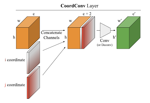

 denotes elementwise multiplication, and
  is the sigmoid nonlinearity. In the saturated regime, this parametrization encourages
  , and so a linear combination using this kind of
  , tends to behave like an addition or subtraction of its inputs (without scaling). In light of the preceding discussion, it is important to note here again that the model does not force this kind of behavior, but rather it merely facilitates it.
 ), is defined in terms of equivalence classes of sequences of real numbers. Two sequences of real numbers,
  and
and  , are considered equal (hence represent the same hyperreal number) iff the set of indices where they agree,
  , is quasi-big. The technical definition of a quasi-big set is somewhat complicated, but the most important properties of quasi-big sets can be listed as follows:
 and
and  are quasi-big sets, then so is
  .
. , then
  , i.e. hyperreals strictly contain the reals (we map any real
  to the equivalence class containing the sequence
  ).
). such that
  , yet
, yet  for every positive real number
  ).
). that is expressive enough to develop the entire calculus in, any given sentence is true with respect to
  iff it is true with respect to
  is a real number, then
  is also infinitesimal. Moreover, if
  and
and  are infinitesimals, then so are
  and
and  .
. is an infinite hyperreal.
 greater than
  and
and  are infinitely close, denoted by
  , if
, if  is infinitesimal or zero.
 is nonstandard if
  (or
(or  ) is nonstandard.
 to be continuous at
  implies
  . In
. In  -type argument.
 is defined as:
 , than models that don’t generalize well. The Jacobian norm at a given point can be considered as an estimate of the average sensitivity of the model to perturbations around that point. So, similar to Morcos et al.’s observation, this result amounts to a correlation between the model’s generalization performance and a particular measure of its noise robustness.
  , where
  is a data-dependent posterior distribution over the “hypotheses” (think of a distribution over neural network parameters) specific to a learning algorithm and training data
  and
and  is a data-independent prior distribution over the hypotheses. The main challenge in coming up with useful bounds in this framework is finding a good prior
  -divergence between the prior and the posterior in the bound. This basically requires guessing what kinds of structure are favored by the training algorithm, training data and model class we happen to use (previously, Dziugaite & Roy had directly minimized the PAC-Bayes bound with respect to the posterior distribution instead of guessing an appropriate prior, assuming a Gaussian form with diagonal covariance for the posterior, and came up with non-vacuous and fairly tight bounds for MNIST models. Although this is a clever idea, it obscures which properties of trained neural nets specifically lead to better generalization).
 and
and  , where
  denotes the number of bits required to describe the model
  denotes the compressed version of the trained model, we get a bound like the following (Theorem 4.1 simplified):
 , whereas their compressed model achieves an actual error of
  on the validation data.
 matrix containing the log-probability of each word in the vocabulary given each context in the dataset:
  , where
  is the number of all distinct contexts in the dataset and
  is the vocabulary size;
  is an
is an  matrix containing the embedding space representations of all distinct contexts in the dataset, where
  is the dimensionality of the embedding space; and
  matrix containing the softmax weights.
 and
and  , so
, so  (we’re assuming that
  , using the notation above), so there is no “bottleneck” due to a dimensionality difference between the input and output spaces. Mathematically, the layer is described by the equation:
  , where
  is relu and we ignore the biases for simplicity. The weights,
  , over a bunch of inputs. The result is shown by the blue line (labeled “Dense”) below:
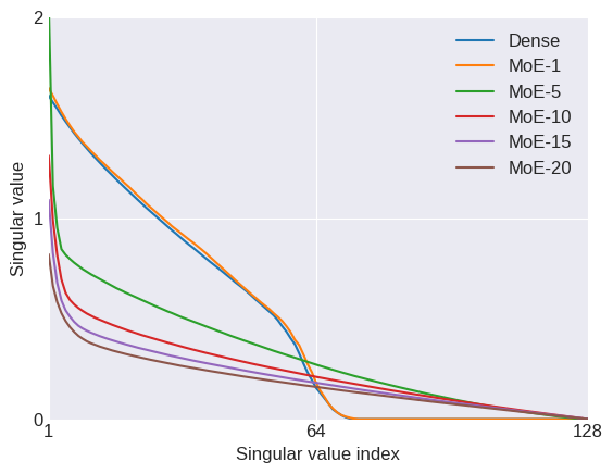
 of the singular values would have been degenerate (as opposed to roughly half in this example), but this is just a single layer and degeneracy can increase sharply in deeper models (again see
 denotes the number of experts,
  represents the gating model for the
  is the
  are softmax functions (with the additional difference that in their model the input
  , already effectively breaks the degeneracy:
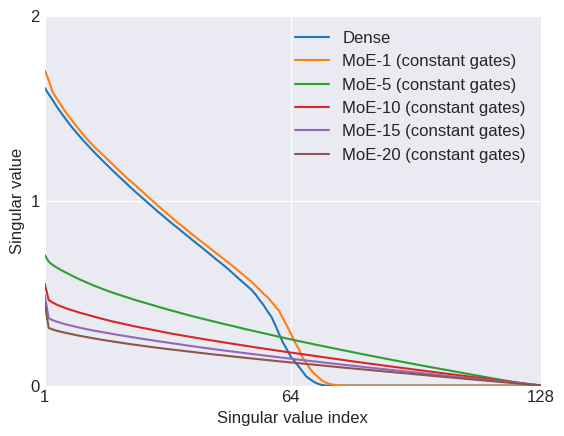

 and expert model
  – and a feature dimension -implicitly represented by the vectors
  etc.-), hence the inductive biases implemented by this model are not exactly the same as in the flat dense case above, but the analogy suggests that part of the success of this model may be explained by degeneracy breaking as well.
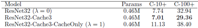
 ) is the baseline model without a cache component, ResNet32-Cache3 is a model that linearly combines the predictions of the cache component and the baseline model (as you may have guessed,
  represents the mixture weight of the cache component), and ResNet32-Cache3-CacheOnly (
 ) is a model that uses the predictions of the cache component only.
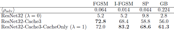
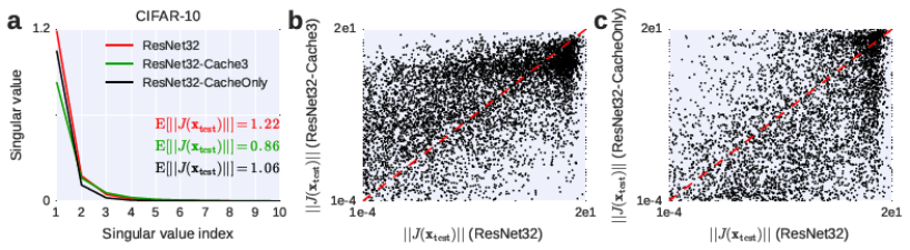
 and
and  , their composition is represented by the pair
  where:
 and
and 
 and
and  are parameters shared across all compositions and optimized for a particular task, e.g. sentiment prediction.
![[a, \alpha]](https://s0.wp.com/latex.php?latex=%5Ba%2C+%5Calpha%5D&bg=ffffff&fg=404040&s=0&c=20201002) where the first part of the vector
where the first part of the vector  captures the content semantics, and the second part
  captures the operator semantics. After composing two words,
 ![[b, \beta]](https://s0.wp.com/latex.php?latex=%5Bb%2C+%5Cbeta%5D&bg=ffffff&fg=404040&s=0&c=20201002) , we get the following content and operator parts:
, we get the following content and operator parts: and
and 
 with a more general function
  , which can be a shallow MLP, for instance. The important point is to note that
  and
and  , is represented by their circular convolution. Because convolution corresponds to product in the Fourier domain, we can express this as the inverse transform of the elementwise multiplication of the discrete Fourier transforms of the vectors:
![\mathbf{a} \circledast \mathbf{b} = \mathcal{F}^{-1}([r_1s_1 \exp(i(\phi_1 + \chi_1)), \ldots, r_ns_n \exp(i(\phi_n + \chi_n))])](https://s0.wp.com/latex.php?latex=%5Cmathbf%7Ba%7D+%5Ccircledast+%5Cmathbf%7Bb%7D+%3D+%5Cmathcal%7BF%7D%5E%7B-1%7D%28%5Br_1s_1+%5Cexp%28i%28%5Cphi_1+%2B+%5Cchi_1%29%29%2C+%5Cldots%2C+r_ns_n+%5Cexp%28i%28%5Cphi_n+%2B+%5Cchi_n%29%29%5D%29&bg=ffffff&fg=404040&s=0&c=20201002)
![\tilde{\mathbf{a}} = [r_1 \exp(i \phi_1), \ldots, r_n \exp(i \phi_n)]](https://s0.wp.com/latex.php?latex=%5Ctilde%7B%5Cmathbf%7Ba%7D%7D+%3D+%5Br_1+%5Cexp%28i+%5Cphi_1%29%2C+%5Cldots%2C+r_n+%5Cexp%28i+%5Cphi_n%29%5D&bg=ffffff&fg=404040&s=0&c=20201002) representing the discrete Fourier transform of
representing the discrete Fourier transform of ![\tilde{\mathbf{b}} = [s_1 \exp(i \chi_1), \ldots, s_n \exp(i \chi_n)]](https://s0.wp.com/latex.php?latex=%5Ctilde%7B%5Cmathbf%7Bb%7D%7D+%3D+%5Bs_1+%5Cexp%28i+%5Cchi_1%29%2C+%5Cldots%2C+s_n+%5Cexp%28i+%5Cchi_n%29%5D&bg=ffffff&fg=404040&s=0&c=20201002) representing the discrete Fourier transform of
representing the discrete Fourier transform of 
 associated with an item
  (which can be thought of as the “key” associated with
 ![\tilde{\mathbf{a}^{-1}} = [s_1^{-1} \exp(-i \chi_1), \ldots, s_n^{-1} \exp(-i \chi_n)]](https://s0.wp.com/latex.php?latex=%5Ctilde%7B%5Cmathbf%7Ba%7D%5E%7B-1%7D%7D+%3D+%5Bs_1%5E%7B-1%7D+%5Cexp%28-i+%5Cchi_1%29%2C+%5Cldots%2C+s_n%5E%7B-1%7D+%5Cexp%28-i+%5Cchi_n%29%5D&bg=ffffff&fg=404040&s=0&c=20201002) :
:
 grows linearly with the number of items (or associations) in memory and will be small if the keys are chosen sufficiently orthogonally (in the paper, only random normal keys are considered; however, orthogonal keys would be better, since although any pair of random normal keys are likely to be orthogonal, linear dependencies between a number of such keys also become highly likely; orthogonal keys, on the other hand, eliminate such linear dependencies as well).
 in this scheme. We can, for instance, do something like:
  .
. with
with  on top, we can do
  where
where  is an arbitrary vector. Then, we can define push and pop operations on this stack as follows:
 (push item
  )
) (return the top item)
 (pop the top item)
 , we can chunk it into smaller sequences as follows:


 .
. ,
, and
and  represent the thematic roles of “agent” and “object” for the eat frame, respectively.
 .
. , where
  denotes the unique identifier for “Mark”.
 and
and  , are introduced as linear functions of the inputs and hidden states (analogous to gates in standard LSTMs, but without the nonlinearity). The cell state is then updated as follows:

 is a new nonlinearity they introduce. The only difference from the standard LSTM equations is the convolution with the input and output memory keys,
 is the synaptic modification made at time
  and
and  is the weighting function that determines the effect of a modification made at time
  , that arrive at the synapse at a constant rate and are uncorrelated across time. It is assumed that there are

 we can afford before the variance term diverges is
  (to see this, note that plugging this in the denominator gives the harmonic series). One can make this argument more formal by writing down an objective (e.g. the area under the
  curve above an arbitrary threshold), optimizing with respect to
  decay can achieve the almost extensive
  memory capacity (capacity is defined as the time at which the
  in the paper).
 is the diffusion coefficient (where
  is known as the heat capacity and
  is the conductivity). Recall that the solution to the heat equation at
  already displays the required
  variables) to achieve the
  and an exponentially decreasing conductivity
  . This has the effect of slowing down the diffusion along the
  variables to implement the desired
  decay in a discretized version.
 discrete variables required in the linear model could be improved upon in a nonlinear model, or perhaps the robustness of the model could be improved with a nonlinear model, or perhaps a nonlinear model could perform better than any linear model under more realistic scenarios not studied in this paper.
 initialization. The training loss decreases rapidly at first, but then quickly asymptotes at a suboptimal value. The gradients certainly don’t vanish (or explode), at least initially! They do become smaller as training progresses, but that is to be expected and it’s not clear at all that the gradients here are “too small” in any sense:
 matrix (initialized with the standard
 in the following example) and deliberately create vanishing gradient norms in the initial network without much effect on the training performance (magenta):
 parameters, as in the above examples, but in reality you’re effectively fitting a model with substantially fewer degrees of freedom because of the degeneracies. So, the problem with the “Fold 0” and “Fold 1” networks above was that although the gradient norms are fine, the network’s available degrees of freedom contribute extremely unevenly to those norms: while a handful of degrees of freedom (non-degenerate ones) explain almost all of it, the vast majority (degenerate ones) don’t contribute anything at all (a conceptually helpful, but not strictly accurate, way of thinking about this may be to imagine only a few of the hidden units in each layer changing their activity in response to different inputs, while the vast majority just responding the same way independently of the input).
 , except for a vanishingly small fraction of singular values that become arbitrarily large. This result isn’t just relevant for linear networks. A similar thing happens in nonlinear networks too: as depth increases, the responses of the hidden units in a given layer become increasingly lower-dimensional, i.e. increasingly degenerate. In fact, this “degeneration process” can proceed much more quickly with depth in nonlinear networks with hard-saturating boundaries as in ReLU networks.
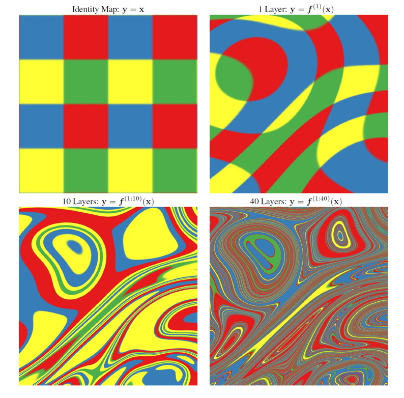 As depth increases, the input space (shown on the top left) gets distorted into increasingly thin filaments with only a single direction (orthogonal to the filament) at each point in the input space affecting the network’s response (it may be a bit hard to extrapolate from this figure how input spaces of more than two dimensions will behave under a similar mapping, but it turns out they become “hyper-pancakey” locally, i.e. there is a single direction at each point, orthogonal to the pancake surface, the network is sensitive to). Along that sensitive direction, the network in fact becomes hyper-sensitive to variations.
 . If points are interpreted as points and lines as great circles on the surface of the sphere, the parallel postulate is violated, because any two great circles on the surface of the sphere have to intersect, hence they are not parallel. However, the problem with this model is that it also violates the second axiom: line segments cannot be extended indefinitely, since great circles are closed curves. So, it was not taken seriously as a plausible model of plane geometry.
 . The points in

 , consisting of the complex plane and a single point at infinity.
 , we define a circle to be either a Euclidean circle in
  or a Euclidean line in
  . We denote the group of homeomorphisms of
  . Our first job is to exactly characterize this group. For this purpose, we first define the Möbius transformations.
 of the following form:
 where
where  and
and  .
. .
. , is called the general Möbius group and denoted by
  .
. .
. .
. and
and 
 where
where  are purely imaginary and, again,
 ![f: [a,b] \rightarrow \mathbb{R}^2](https://s0.wp.com/latex.php?latex=f%3A+%5Ba%2Cb%5D+%5Crightarrow+%5Cmathbb%7BR%7D%5E2&bg=ffffff&fg=404040&s=0&c=20201002) define a path in the Euclidean plane. The Euclidean length of
define a path in the Euclidean plane. The Euclidean length of 
 is called the Euclidean line element. A more general line element can be defined by scaling the Euclidean line element by a scale factor,
  , that could depend on
  : i.e.
  . We define the length of
 for all
  and all

 defined in the interval
 ![[a,b]](https://s0.wp.com/latex.php?latex=%5Ba%2Cb%5D&bg=ffffff&fg=404040&s=0&c=20201002) . Then,
. Then,  . We see that the length blows up as
  .
. The idea is to find a
  that maps the hyperbolic line passing through
  and
and  to the imaginary axis so that
  and
and  for some
  and
and  :
:
 and
and  are the coordinates of
  and
and  .
. , whereas for the latter case,
  . Therefore, ultraparallel lines behave more like parallel lines in Euclidean space.
 A hyperbolic line in
  of a hyperbolic line in
  is an element of
  This implies that hyperbolic lines in
  (
(
 , then define lengths and distances based on this

![f: [0,r] \rightarrow \mathbb{D}](https://s0.wp.com/latex.php?latex=f%3A+%5B0%2Cr%5D+%5Crightarrow+%5Cmathbb%7BD%7D&bg=ffffff&fg=404040&s=0&c=20201002) ,
,  . Then,
  . Again, we see that the length blows up as
  .
. .
. :
:
 by:
by:
 is also invariant under the action of the group
 . This implies that for a disk with center 0 and radius
  as
as  . This is very unlike the Euclidean case, where
  as
as  with interior angles
  , the area is given by
  .
. , then the area of
 . The situation is completely different in the hyperbolic plane: for all
  and each
  , there is a compact regular hyperbolic
  .
. 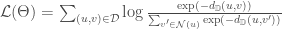
 denotes the set of items unrelated to
  , and
, and  denotes the hyperbolic distance between the embeddings of the items in the Poincaré ball model.
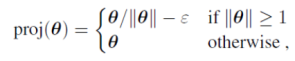
 ensures numerical stability.
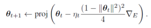
 is the learning rate,
  is the Euclidean gradient and the term
 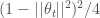 is just the inverse of the metric, which in turn is just the square of the scaling factor
  derived above for the Poincaré disk model.
 ):
):![\mathbf{h}_{t+1} = f\Big( \mathcal{LN}\Big[\mathbf{W}_h \mathbf{h}_t + \mathbf{W}_x \mathbf{x}_t + \big(\eta \sum_{\tau=1}^{\tau=t-1}\lambda^{t-\tau-1}\mathbf{h}_\tau \mathbf{h}_\tau^{\top}\big) f(\mathbf{W}_h \mathbf{h}_t + \mathbf{W}_x \mathbf{x}_t) \Big] \Big)](https://s0.wp.com/latex.php?latex=%5Cmathbf%7Bh%7D_%7Bt%2B1%7D+%3D+f%5CBig%28+%5Cmathcal%7BLN%7D%5CBig%5B%5Cmathbf%7BW%7D_h+%5Cmathbf%7Bh%7D_t+%2B+%5Cmathbf%7BW%7D_x+%5Cmathbf%7Bx%7D_t+%2B+%5Cbig%28%5Ceta+%5Csum_%7B%5Ctau%3D1%7D%5E%7B%5Ctau%3Dt-1%7D%5Clambda%5E%7Bt-%5Ctau-1%7D%5Cmathbf%7Bh%7D_%5Ctau+%5Cmathbf%7Bh%7D_%5Ctau%5E%7B%5Ctop%7D%5Cbig%29+f%28%5Cmathbf%7BW%7D_h+%5Cmathbf%7Bh%7D_t+%2B+%5Cmathbf%7BW%7D_x+%5Cmathbf%7Bx%7D_t%29+%5CBig%5D+%5CBig%29+&bg=ffffff&fg=404040&s=0&c=20201002)
![\mathcal{LN}[\cdot]](https://s0.wp.com/latex.php?latex=%5Cmathcal%7BLN%7D%5B%5Ccdot%5D&bg=ffffff&fg=404040&s=0&c=20201002) refers to
refers to  .
.![\mathbf{h}_{t+1} = f\Big( \mathcal{LN} \Big[ \big[\mathbf{W}_{h} + \eta \sum_{\tau=1}^{\tau=t-1}\lambda^{t-\tau-1}\mathbf{h}_\tau \mathbf{h}_\tau^{\top} \big] \mathbf{h}_{t} + \mathbf{W}_{x} \mathbf{x}_{t} \Big] \Big)](https://s0.wp.com/latex.php?latex=%5Cmathbf%7Bh%7D_%7Bt%2B1%7D+%3D+f%5CBig%28+%5Cmathcal%7BLN%7D+%5CBig%5B+%5Cbig%5B%5Cmathbf%7BW%7D_%7Bh%7D+%2B+%5Ceta+%5Csum_%7B%5Ctau%3D1%7D%5E%7B%5Ctau%3Dt-1%7D%5Clambda%5E%7Bt-%5Ctau-1%7D%5Cmathbf%7Bh%7D_%5Ctau+%5Cmathbf%7Bh%7D_%5Ctau%5E%7B%5Ctop%7D+%5Cbig%5D+%5Cmathbf%7Bh%7D_%7Bt%7D+%2B+%5Cmathbf%7BW%7D_%7Bx%7D+%5Cmathbf%7Bx%7D_%7Bt%7D+%5CBig%5D+%5CBig%29&bg=ffffff&fg=404040&s=0&c=20201002)
 and the representation
  , i.e.
  and representation compression becomes minimizing the mutual information between the input
  and the representation
  . The authors seem to imply that the compression phase is essential to understanding successful generalization in deep neural networks.
 even mean?–. So, I did something that seemed most reasonable to me, namely computed the norms of the mean and standard deviation (std) of gradients (across a number of mini-batches) at each epoch. Comparing these two should give an indication of the relative size of the mean gradient compared to the size of the noise in the gradient. The dynamics seems to be always diffusion (noise) dominated with no qualitatively distinct phases during training:
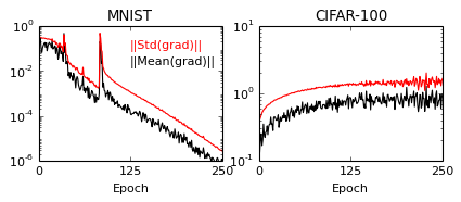
![[-1,1]](https://s0.wp.com/latex.php?latex=%5B-1%2C1%5D&bg=ffffff&fg=404040&s=0&c=20201002) into equal-length bins. But then the whole thing basically depends on the discretization and it’s not even clear how this would work for unbounded ReLU units.
into equal-length bins. But then the whole thing basically depends on the discretization and it’s not even clear how this would work for unbounded ReLU units. is a subset of the abelian group
  . We define the subgroup of
  generated by
 borrowed from
  is indeed a group).
  for some finite subset
  , i.e.
  for some
  for all smaller
  . If
. If  is torsion subgroup. The rank of
  , to be a nonsingular cubic curve containing at least one point with
  . It isn’t a trivial assumption to assume that such a point exists. For example, it isn’t at all obvious that a given homogeneous cubic polynomial with rational coefficients should have a solution with rational coordinates.
 be two points on
  . We define
  as follows: first let
  . Then draw the line
  connecting
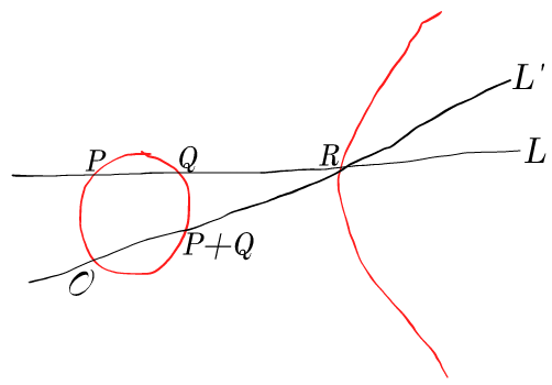
 , which is an easy-to-compute algebraic function of the coefficients describing the curve. The curve is singular if and only if
  .
. , i.e.
  , and especially in the size of
  .
.  .
. turns out to be so important that it gets its own name,
  , so Hasse’s theorem can be restated as saying that
  .
. , and we can say a few things about the group structure of
  is also finitely generated, hence is finite.
 or
or  . I fact,
  and
and  , where the order of
  , with
  integers, if
  and
and  are integers and either
  , in which case
  , or else
 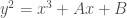 , where
  is 6, because the monomial with the largest degree, i.e.
  , has degree 6. The second notion of degree is purely geometric: informally, we want to say that the geometric degree of a curve described by a polynomial equation
  is the number of intersection points it has with an arbitrary line
 is an algebraically closed field means that any non-constant polynomial whose coefficients are in
  has no roots in
  does not even make sense in
  . Setting
  gives us the usual (“finite”) plane. Points with
  correspond to “points at infinity”. The coordinates
  with
with  describe the same point. So, the points at infinity form a single line at infinity that can be parametrized by
  or by
or by  where
where  in two variables,
  , this means multiplying each monomial in
  is
is  . Now, to find out which points at infinity get attached to the curve described by the polynomial equation
  , we simply set
  to which the solutions are
  with
with  . By the property above, these describe a single point which we might as well denote by
  .
. . Then
  obtained by plugging the parametric form of
  . This definition was a mouthful, so let’s do an example: suppose our curve is defined by the polynomial
  and the line
  and
and  . If we plug these in
  . The root
  has multiplicity
  is defined to be
  ), without having to worry about whether the standard analytic definition in terms of limits even makes sense in a given field. Ditto for partial derivatives.
 , as you can easily check.
 are two projective curves that intersect at a finite number of points:
  ,
,  ,
,  ,
,  . Then Bézout’s theorem states that the product of the degrees of the homogeneous polynomials defining
  , i.e. the sum of the multiplicities of all intersection points. The fact that any line intersects a curve